Quantifying the minimum ensemble size
for asymptotic accuracy
of the ensemble Kalman filter
using the degrees of instability
* This is joint work with Dr. Miyoshi (Team Principal)
Nagoya University, Japan
* The author was supported by RIKEN Junior Research Associate Program and JST SPRING JPMJSP2110.
\Psi
\Psi
Kota Takeda
Self-introduction
Kota Takeda

Assistant Prof.
at Nagoya Univ., Japan
Research topics:
Uncertainty Quantification
Fluid mechanics
Data assimilation
Nagoya

Contents
-
Introduction
- Prediction, m^*, accuracy, Our contributions
-
Background
-
State estimation by EnKF
- Mathematical formulation, Ensemble Kalman filter, accuracy
-
Dynamical instability
- LEs, Unstable subspace literature, Conjecture
-
State estimation by EnKF
- Our approach
-
Numerical Result
- Result supporting the conjecture
- Summary
Numerical Weather Prediction
Introduction
Prediction is Hard
(Insert Image: Past Slide p.6 - Typhoon/Chaos)
- Chaos: Sensitivity to initial conditions makes long-term prediction impossible. -> need ensemble to estimate uncertainty
- Goal: Estimate the true state from noisy observations to initialize forecasts.
Note: As we all know, weather prediction is difficult due to chaos. We use data assimilation to estimate the current state.
Note: As we all know, weather prediction is difficult due to chaos. We use data assimilation to estimate the current state.
Note: As we all know, weather prediction is difficult due to chaos. We use data assimilation to estimate the current state.
Unpredictable in long-term
Numerical Weather Prediction
State estimation of High dimensional chaotic system

Numerical Weather Prediction
Numerical Weather Prediction
State estimation of High dimensional chaotic system
Unpredictable in long-term

e.g., Typhoon forecast circles
\sim 10^8
3D grid × variable
Numerical Weather Prediction
Numerical Weather Prediction
State estimation of High dimensional chaotic system

\sim 10^8
3D grid × variable
→ Estimating uncertainty in prediction by ensemble
Fundamental Problem
- EnKF is standard for high-dimensional geophysical systems .
-
Constraint: Ensemble size ($m$) is limited by computational cost.
- Real systems: $N_x \sim 10^9$, $m \sim 100$.
- Risk: Small $m$ leads to Filter Divergence.
- Question: What is the theoretical minimum $m$ to guarantee "accuracy"?
Orange: Estimate
State estimation by EnKF
Large ensemble
Small ensemble
Success
Failed
(Filter divergence)
Green: True state
Formulation of accuracy: why focus on Noise Scaling?
-
(Standard) Fixed Noise ($r$) Analysis:
Vary $m^*$ depending on $r$
Hard to distinguish accuracy similar with the observation noise level. -
(Our) Asymptotic ($r \to 0$) Analysis:
- Convergent: Error $\propto r^2$ (Slope 2).
- Divergent: Error $\approx O(1)$ (Flat).
(Insert Image: Past Slide p.26 - Log-Log Schematic)
Fig: Schematic of Noise-scaled Accuracy
Note: Instead of looking at a fixed noise level, we look at the scaling behavior as noise goes to zero. This gives us a sharp, qualitative distinction between success and failure.
Our Contributions
- Reformulation: "Noise-scaled filter accuracy" ($r$-asymptotic accuracy).
- The Conjecture: Minimum size is determined by "positive Lyapunov exponents": $$m^* = N_+ + 1$$
- Methodology: "Ensemble spin-up and downsizing" strategy.
Note: We propose that $N_+$ is the key number.
Background
Notation: model dynamics

\mathbb{R}^{N_x}
t
\frac{d \boldsymbol{x}}{dt} = \boldsymbol{f}(\boldsymbol{x})
(\boldsymbol{f}: \mathbb{R}^{N_x} \rightarrow \mathbb{R}^{N_x}, \boldsymbol{x}(0) = \boldsymbol{x}_0 \in \mathbb{R}^{N_x})
\boldsymbol{x}(t) = \boldsymbol{\Psi}_t (\boldsymbol{x}_0)
Continuous-time
Evolution map
(\boldsymbol{\Psi}_t : \mathbb{R}^{N_x} \rightarrow \mathbb{R}^{N_x}, t \ge 0)
\boldsymbol{x}_{t_1}
\boldsymbol{x}(t+t_1)
\boldsymbol{\Psi}_t
Discrete-time
\boldsymbol{x}_n = \boldsymbol{\Psi} (\boldsymbol{x}_{n-1})
\boldsymbol{\Psi} = \boldsymbol{\Psi}_\tau \ (\text{for fixed } \tau > 0)
from
\boldsymbol{y}_{1:n} = \{\boldsymbol{y}_i \mid i \le n\}
Filtering problem
\boldsymbol{x}_n
Estimate
n \in \mathbb{N},
known:
\boldsymbol{\Psi},
H,
Obs. up to now
True
Obs.
Estim.
\mathbb{R}^{N_x}
\mathbb{R}^{N_y}
\mathbb{R}^{N_x}
H
...
\boldsymbol{x}_1
\boldsymbol{x}_2
\boldsymbol{x}_0
\boldsymbol{y}_1
\boldsymbol{y}_2
\boldsymbol{\Psi}
...
\overline{\boldsymbol{x}}_1
\overline{\boldsymbol{x}}_2
\overline{\boldsymbol{x}}_0
...
\boldsymbol{\Psi}
\boldsymbol{\Psi}
\boldsymbol{\Psi} = \boldsymbol{\Psi}_t.
Induced from differential equations:
: Model dynamics
\Psi
State space model
\begin{cases}
\boldsymbol{x}_n = \boldsymbol{\Psi}(\boldsymbol{x}_{n-1}), \\
\boldsymbol{y}_n = H \boldsymbol{x}_n + \boldsymbol{\xi}_n.
\end{cases}
H
: Observation matrix
Assume
H = I.
\boldsymbol{\xi}_n
: Gaussian noise
\sim \mathcal{N}(\boldsymbol{0}, r^2 I).
Filtering Problem
\boldsymbol{\Psi}
\boldsymbol{\Psi}
\boldsymbol{\Psi}
\mathcal{N}(\boldsymbol{0}, r^2 I).
- Estimates by ensemble
- Update:
- Correct mean and covariance
using observations
\mathbb{R}^{N_x}
t
y_1
y_2
t_1
t_2
t_3
\tau
t_0
Repeat (I) & (II)...
(II)Analysis
(I) Forecast
\Psi
\boldsymbol{x}_0^{a(1)}
\boldsymbol{x}_0^{a(m)}
\boldsymbol{x}_0^{a(2)}


\boldsymbol{x}_1^{f(1)}
\boldsymbol{x}_1^{a(1)}

\vdots
\boldsymbol{x}_1^{f(m)}
\boldsymbol{x}_1^{a(m)}
Just evolve each sample
Correct samples based on the least squares
X_{n-1}^a \overset{\text{(I)}}{\rightarrow} X_n^f \overset{\text{(II)}}{\rightarrow} X_n^a
\overline{\boldsymbol{x}}_n = \frac{1}{m} \sum_{k=1}^m \boldsymbol{x}_n^{a(k)}
Estimate
X_n^a = (\boldsymbol{x}_n^{a(k)})_{k=1}^m, \\
X_n^f = (\boldsymbol{x}_n^{f(k)})_{k=1}^m
ensemble
ensemble
(Evensen2009)
Ensemble Kalman filter (EnKF)
How to generate estimates?: EnKF
(I) Forecast
\mathrm{rank}(P_n^f) \le m - 1.
Remark: the rank is restricted as
P_n^f = \operatorname{Cov}_m(\boldsymbol{X}_n^f).
Estimate forecast uncertainty using eigenvalues and vectors of forecast covariance:
(II) Analysis
Stronger correction in higher uncertainty along the direction.
→ rank-deficient
m \le N_x
P_n^f
Why ensemble?
→ No correction in the degenerated direction.
\boldsymbol{x}_1^{f(1)}
\boldsymbol{x}_1^{f(3)}
\boldsymbol{x}_1^{f(2)}
\Psi
Multiplicative inflation
"accutual"
\mathrm{trace}({P_n^f})
P_n^f \rightarrow \alpha^2 P_n^f \ (\alpha \ge 1).
Compensate for underestimated variability of forecasts with a limited ensemble.
(*An efficient implementation is used in practice.)
\mathrm{trace}({\alpha^2 P_n^f})
* The rank of covariance is not improved
\mathrm{rank}({P_n^f}) = \mathrm{rank}({\alpha^2 P_n^f})
Covariance inflation
m
ensemble size
Question: minimum ensemble
Question
How many samples are required
for 'accurate state estimation' using EnKF?
m
ensemble size
\mathbb{E}[\mathrm{RMSE}_n] = \mathbb{E}\left[\textstyle{\frac{|\delta_n|}{\sqrt{N_x}}}\right] < r.
Disadvantage
Formulation of accuracy
Question
How many samples are required
for 'accurate state estimation' using EnKF?
The standard accuracy
m
ensemble size
\limsup_{n\rightarrow \infty}\mathbb{E}[|\delta_n|^2] = O(r^2),
(Asymptotic) filter accuracy
\delta_n = u_n - \overline{v}_n
: state estimation error.
r^2
: variance of obs. noise,
where
\overline{v}_n = \textstyle{\frac{1}{m} \sum_{k=1}^m v^{(k)}_n}
estimate of EnKF
r
squared error
log-log
O(r^2)
Formulation of accuracy
Question
How many samples are required
for 'accurate state estimation' using EnKF?
Commonly used in mathematical studies
m
ensemble size
ensemble
Large
m
Accurate
m
Small
m
ensemble
Inaccurate
Advantage:
Qualitative distinction
r
squared error
log-log
O(r^2)
Formulation of accuracy
Question
How many samples are required
for 'accurate state estimation' using EnKF?
← Find minimum
m = m^*
achieving accuracy!
Summary of EnKF
- Mechanism of EnKF <-> dynamical instability
- Question: minimum ensemble size m*
- (Our) Reformulate accuracy
Dynamical instability
Characterizing Instability: The Tangent Linear Model
- Dynamics: $\frac{dx}{dt} = f(x)$.
-
Perturbation Evolution: Let $\delta x(t)$ be an infinitesimal perturbation. $$\frac{d}{dt}\delta x(t) = \mathbf{J}_f(x(t)) \delta x(t)$$
- $\mathbf{J}_f$: Jacobian matrix of $f$.
- Fundamental Matrix $\Phi(t, x_0)$: Maps initial perturbation to time $t$: $\delta x(t) = \Phi(t, x_0) \delta x_0$.
Note: To rigorously define instability, we look at the Tangent Linear Model. The growth of perturbations is governed by the Jacobian along the trajectory.
Dynamical instability
infinitesimal perturbation
D\Psi
expanded
contracted
N_+:
Dim. of unstable directions in tangent sp.
ex) one unstable direction in 3D
Jacobian matrix
Idea: Measuring 'degrees of freedom' of a chaotic system based on sensitivities to small perturbations
→ High uncertainty of prediction along this direction.
Definition of Lyapunov Exponents
- Singular Value Decomposition (SVD): Compute SVD of $\Phi(t, x_0)$ with singular values $\sigma_1 \ge \dots \ge \sigma_{N_x}$.
- Lyapunov Exponents (LEs): $$\lambda_i = \lim_{t\to\infty} \frac{1}{t} \log \sigma_i(\Phi(t, x_0))$$
- Meaning: Asymptotic exponential growth rate of the $i$-th principal axis.
Note: LEs are defined not by eigenvalues, but by the singular values of the propagator. They measure the average exponential expansion or contraction rates over infinite time.
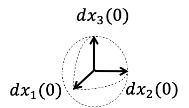
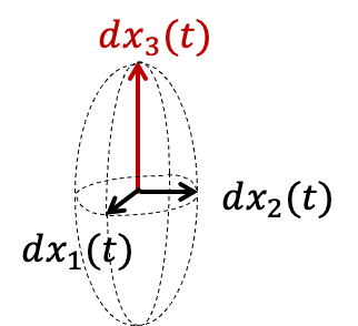
Geometric Interpretation
* Initial error ball evolves into an **ellipsoid**.
* **Expanding axes:** $\lambda_i > 0$ (Unstable).
* **Contracting axes:** $\lambda_i < 0$ (Stable).
(Insert Image: Past Slide p.34 - Ellipsoid Expansion)
Fig: Deformation of phase space volume
Fig: Deformation of phase space volume
Note: Geometrically, an initial error sphere is stretched into an ellipsoid. The directions corresponding to positive exponents expand exponentially. These are the directions we must constrain with data.
N_+:
Dim. of unstable directions in tangent sp.
D\Psi
Jacobian matrix
N_+ := \#\{i \mid \lambda_i > 0\}
Define
Remark positive exponent → unstable
\delta\bm{u}_n^{(i)}
\delta\bm{u}_0^{(i)}
\Psi^n
\Psi^n
|\delta\bm{u}_n^{(i)}| \approx e^{\lambda_i n} |\delta\bm{u}_0^{(i)}|
\sigma_i(A)
:
A
i
-singular value of
Lyapunov exponents:
\lambda_1 \ge \dots \ge \lambda_{N_x}
\lambda_i = \lim_{n \rightarrow \infty} \frac{1}{n} \log \sigma_i(D\Psi^n(\bm{u})).
Definition
Information on
Idea: Measuring 'degrees of freedom' of a chaotic system based on sensitivities to small perturbations
Dynamical instability
Subspace Dimensions & The Conjecture
- $N_+$ (Unstable Subspace): Number of positive LEs ($\lambda_i > 0$).
- $N_0$ (Unstable + Neutral): Number of non-negative LEs ($\lambda_i \ge 0$).
- The Conjecture: $$m^* = N_+ + 1$$ (We hypothesize the Neutral direction does not cause asymptotic divergence).
Note: Usually, people suggest $N_0$. We claim $N_+$ is enough.
Low Dimensionality
Ansatz (low-dimensional structure):
most geophysical flows satisfy
owing to their 'dissipative' property.
N_+ \ll N_x
Low Dimensionality
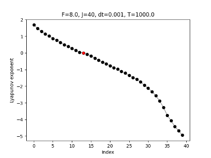
ex) 40-dim. Lorenz 96 model (chaotic toy model)
\lambda_i
i
0
unstable
stable
- Navier-Stokes equations
-
Primitive equations
(core of atmospheric model)
Other dissipative systems
N_+ = 13 \ll 40 = N_x
Lyapunov exponents
(T.+2025)
Ansatz (low-dimensional structure):
most geophysical flows satisfy
owing to their 'dissipative' property.
N_+ \ll N_x
Literature: DA
DA studies have revealed sufficient conditions for .
m
Literature: Math.
(de Wiljes+2018, T.+2024)
(Sanz-Alonso+2025)
(González-Tokman+2013)
m \ge N_x + 1
m \ge 6 N_y
m \ge N_+ + 1
for
using
'Stability' of
\Psi
in unobserved sp.
\Psi
'Lipschitz'
using
too many
additional factor
Accurate initial ensemble aligning with the unstable subspace.
Mathematical analyses have revealed sufficient conditions for .
m
Literature: Math.
(de Wiljes+2018, T.+2024)
(Sanz-Alonso+2025)
(González-Tokman+2013)
m \ge N_x + 1
m \ge 6 N_y
m \ge N_+ + 1
for
using
'Stability' of
\Psi
in unobserved sp.
\Psi
'Lipschitz'
using
too many
additional factor
Accurate initial ensemble aligning with the unstable subspace.
unrealistic (should be relaxed)
Mathematical analyses have revealed sufficient conditions for .
m
Focus on
Exploiting Low Dimensionality
Conjecture the minimum ensemble size for filter accuracy with the EnKF is
m^* = N_+ + 1.
(※ with any initial ensemble)
González-Tokman+2013 assume this.
→ How to obtain?
\Psi
\Psi
Tracking only the unstable directions
unstable direction
: critical small ensemble
Exploiting Low Dimensionality
Efficient & Accurate Weather Prediction
Conjecture the minimum ensemble size for filter accuracy with the EnKF is
m^* = N_+ + 1.
(※ with any initial ensemble)
Ansatz
N_+ \ll N_x
m \ll N_x
r
squared error
log-log
O(r^2)
EnKF with
N_{spinup}
: 小
m
: 大
m_0
パラメータ
N_{spinup}
:spin up期間
m_0
:最初のアンサンブル数
m
:削減後のアンサンブル数
n
ねらい:最初は多数のアンサンブルを使うことで真値に近く,不安定方向を向いた「良い」アンサンブルを構成.
Ensemble reduction
でアンサンブル数を削減.
SVD/PCAに基づき共分散行列を低ランク近似.
n=N_{spinup}
\mathbb{R}^{N_u}
0
How to obtain?
Algorithm: Downsizing
At step $n = N_{spinup}$:
- Take ensemble perturbations $V \in \mathbb{R}^{N_x \times m_0}$.
- Compute SVD: $V = U \Sigma W^T$.
- Retain leading $m$ singular vectors: $$V_{new} = U[:, 1:m] \Sigma[1:m, 1:m]$$.
Result: Efficient ensemble aligned with instability.
Note: This ensures that when we test $m=14$, for example, those 14 members are the "best possible" 14 members, capturing the most variance.
Require:Why Spin-up Works? (Alignment)
(Insert Image: Past Slide p.38 - Ensemble Alignment)
- Natural Alignment: Random perturbations naturally align with the Unstable Subspace (Backward Lyapunov Vectors) over time.
-
Strategy: Spin-up with large $m$, then downsize.
- Ensures $V^f$ captures the unstable subspace efficiently.
Note: Why do we use spin-up? Because the dynamics naturally rotate the ensemble into the unstable subspace. This gives us an "optimal" initialization for testing the limit.
Summary: Dynamical instability
- Characterize instability via LEs
- key: ensemble alignment connects LEs and m*
- (Our) Proposing method
Numerical Result
Supporting the conjecture
Experimental Setup
- Model: Lorenz 96 ($N_x = 40$).
- DA algorithm: ETKF (one of EnKF)
-
Settings:
- Full observation ($H=I$).
- Regimes: $F=8$ and $F=16$.
- Metric: Log-log slope of Squared Error vs. Noise Variance $r^2$.
Numerical Result
To support the conjecture, we perform numerical experiments estimating synthetic data generated by the Lorenz 96 model.
Setup (T.+2025)
obs.:
N_u=40, F=8.0
model:Lorenz96 ( )
H=I
\eta_n \sim N(0, r^2 I), r > 0
noise:
EnKF:
m = 12, 13, \dots, 18
(others are chosen appropriately)
dt = 0.01
numerical integration: RungeKutta
obs. interval:
5
N_+ = 13
N_{steps} = 72000
For each , we compute the dependency of the worst error
on .
\limsup_{n \rightarrow \infty} \mathbb{E}[|\delta_n|^2]
m
r
Model
To support the conjecture, we perform numerical experiments estimating synthetic data generated by the Lorenz 96 model.
Model
To support the conjecture, we perform numerical experiments estimating synthetic data generated by the Lorenz 96 model.
\frac{du^i}{dt} = (u^{i+1} - u^{i-2}) u^{i-1} - u^i + f
\bm{u} = (u^i)_{i=1}^{N_x} \in \mathbb{R}^{N_x}, f \in \R,
(Lorenz1996, Lorenz+1998)
u^0 = u^{N_x}, u^{-1} = u^{N_x-1}, u^{N_x + 1} = u^1.
Mimics chaotic variation of
physical quantities at equal latitudes.
u
non-linear conserving
linear dissipating
forcing
Lorenz 96 model
(i = 1, \dots, N_x),
Model
To support the conjecture, we perform numerical experiments estimating synthetic data generated by the Lorenz 96 model.
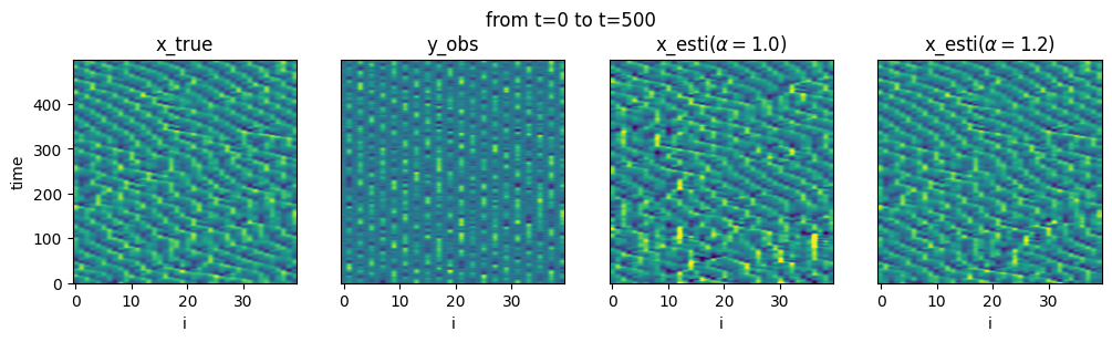
Spatio-temporal plot
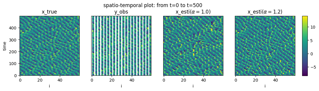
u^{i}(t)
Case 1: $F=8$ (Lyapunov Spectrum)
(Insert Image: Past Slide p.37 - Spectrum F=8)
- Result: 13 Positive Exponents ($N_+ = 13$).
- Prediction: Minimum size should be $m^ = 14$*.
Note: For F=8, we have 13 positive exponents. Note that N_x is 40, so the instability is low-dimensional.
Case 1: $F=8$ (Accuracy Scaling)
(Insert Image: Past Slide p.47 - Scaling F=8 with highlight)
- $m \ge 14$ (Red/Gray): Convergent (Slope $\approx 2$).
- $m < 14$ (Blue): Divergent (Flat).
- Conclusion: The boundary is exactly at $N_+ + 1$.
Note: Here is the main result. Look at the slope. m=12, 13 are flat (divergent). m=14 and above follow the O(r^2) line. The theory holds.
Case 1: $F=8$ (Ensemble spin-up effect1)
(Insert Image: Fig.3 in manuscript)
$m=14$ (border size)
- w/ Spin-up: fast Convergent.
- w/o Spin-up: slow Convergent.
- Conclusion: Spin up suppress slow-convergence
Case 1: $F=8$ (Ensemble spin-up effect2)
(Insert Image: Fig.4 in manuscript)
$m=14$ (border size), mean-accurate init.
- w/ Spin-up: fast Convergent.
- w/o Spin-up: first divergent then slow Convergent.
- Conclusion: Spin up ensemble alignment
Numerical Result
O(r^2)
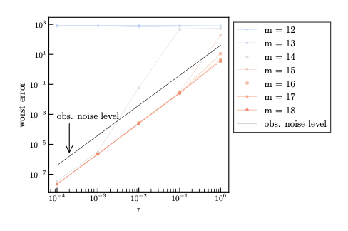
blue
(m <= N_+)
red
(m >= N_+ + 2)
gray
(m = N_+ + 1)
For each , we compute the dependency of the worst error
on → log-log plot.
m
r
r
N_+ = 13
Numerical Result
O(r^2)
O(r^2)
r
blue
(m <= N_+)
red
(m >= N_+ + 2)
gray
(m = N_+ + 1)
For each , we compute the dependency of the worst error
on → log-log plot.
m
r
N_+ = 13
Numerical Result
O(r^2)
O(r^2)
blue
(m <= N_+)
red
(m >= N_+ + 2)
gray
(m = N_+ + 1)
N_+ + 1
accurate
→ This supports the conjecture.
Inaccurate
r
For each , we compute the dependency of the worst error
on → log-log plot.
m
r
N_+ = 13
(filter accuracy)
Case 2: $F=16$ (Higher Instability)
(Insert Image: Paper Fig 5 - Spectrum F=16)
(Insert Image: Paper Fig 6 - Scaling F=16)
- Spectrum: $N_+ = 15$.
- Result: Accuracy achieved at $m \ge 16$.
- Consistency: The rule $m^* = N_+ + 1$ holds for different instability regimes.
Note: We repeated this for F=16. The threshold moved exactly to 16, matching the number of positive exponents plus one.
Summary
New framework:
$r$-asymptotic filter accuracy
$$ \limsup_{n\rightarrow \infty}\mathbb{E}[\mathrm{SE}_n] = O(r^2)$$
distinguishes convergence/divergence qualitatively.
Main Finding:
The minimum ensemble size is given by
$$m^* = N_+ + 1$$
(numerically verified for Lorenz 96 with).
New supporting method:
The ensemble downsizing for faster alignment of the ensemble with the unstable space.
ensemble
Future work
Future work
Numerical studies: Further experiments validating for high-dimensional & complex systems with multi. zero LEs.
Theoretical analysis: Mechanism of ensemble alignment in the spin-up period.
Extension: Extending this theory to localized methods.
Paper: K.T. and T. Miyoshi (preprint), Quantifying the minimum ensemble size for asymptotic accuracy of the ensemble Kalman filter using the degrees of instability.
Thank you
Code: github.com/KotaTakeda/enkf_ensemble_downsizing
Thank you for your attention

Visit my website!
(T.+2024)
K. T. and T. Sakajo, SIAM/ASA Journal on Uncertainty Quantification, 12(4), 1315–1335,
(T.+2025)
K. T. and T. Miyoshi, EGUsphere preprint, https://egusphere.copernicus.org/preprints/2025/egusphere-2025-5144/.
References
- (T.+2024) K. T. & T. Sakajo, SIAM/ASA Journal on Uncertainty Quantification, 12(4), 1315–1335.
- (T. 2025) Kota Takeda, Error Analysis of the Ensemble Square Root Filter for Dissipative Dynamical Systems, PhD Thesis, Kyoto University, 2025.
- (Kelly+2014) D. T. B. Kelly, K. J. H. Law, and A. M. Stuart (2014), Well-posedness and accuracy of the ensemble Kalman filter in discrete and continuous time, Nonlinearity, 27, pp. 2579–260.
- (Al-Ghattas+2024) O. Al-Ghattas and D. Sanz-Alonso (2024), Non-asymptotic analysis of ensemble Kalman updates: Effective dimension and localization, Information and Inference: A Journal of the IMA, 13.
- (Tong+2016a) X. T. Tong, A. J. Majda, and D. Kelly (2016), Nonlinear stability and ergodicity of ensemble based Kalman filters, Nonlinearity, 29, pp. 657–691.
- (Tong+2016b) X. T. Tong, A. J. Majda, and D. Kelly (2016), Nonlinear stability of the ensemble Kalman filter with adaptive covariance inflation, Comm. Math. Sci., 14, pp. 1283–1313.
- (Kwiatkowski+2015) E. Kwiatkowski and J. Mandel (2015), Convergence of the square root ensemble Kalman filter in the large ensemble limit, Siam-Asa J. Uncertain. Quantif., 3, pp. 1–17.
- (Mandel+2011) J. Mandel, L. Cobb, and J. D. Beezley (2011), On the convergence of the ensemble Kalman filter, Appl.739 Math., 56, pp. 533–541.
References
-
(de Wiljes+2018) J. de Wiljes, S. Reich, and W. Stannat (2018), Long-Time Stability and Accuracy of the Ensemble Kalman-Bucy Filter for Fully Observed Processes and Small Measurement Noise, Siam J. Appl. Dyn. Syst., 17, pp. 1152–1181.
-
(Evensen2009)Evensen, G. (2009), Data Assimilation: The Ensemble Kalman Filter. Springer, Berlin, Heidelberg.
-
(Burgers+1998) G. Burgers, P. J. van Leeuwen, and G. Evensen (1998), Analysis Scheme in the Ensemble Kalman Filter, Mon. Weather Rev., 126, 1719–1724.
-
(Bishop+2001) C. H. Bishop, B. J. Etherton, and S. J. Majumdar (2001), Adaptive Sampling with the Ensemble Transform Kalman Filter. Part I: Theoretical Aspects, Mon. Weather Rev., 129, 420–436.
-
(Anderson 2001) J. L. Anderson (2001), An Ensemble Adjustment Kalman Filter for Data Assimilation, Mon. Weather Rev., 129, 2884–2903.
-
(Reich+2015) S. Reich and C. Cotter (2015), Probabilistic Forecasting and Bayesian Data Assimilation, Cambridge University Press, Cambridge.
-
(Law+2015) K. J. H. Law, A. M. Stuart, and K. C. Zygalakis (2015), Data Assimilation: A Mathematical Introduction, Springer.
References
- (Azouani+2014) A. Azouani, E. Olson, and E. S. Titi (2014), Continuous Data Assimilation Using General Interpolant Observables, J. Nonlinear Sci., 24, 277–304.
-
(Sanz-Alonso+2025), D. Sanz-Alonso and N. Waniorek (2025), Long-Time Accuracy of Ensemble Kalman Filters for Chaotic Dynamical Systems and Machine-Learned Dynamical Systems, SIAM J. Appl. Dyn. Syst., pp. 2246–2286.
-
(Biswas+2024), A. Biswas and M. Branicki (2024), A unified framework for the analysis of accuracy and stability of a class of approximate Gaussian filters for the Navier-Stokes Equations, arXiv preprint, https://arxiv.org/abs/2402.14078.
-
(T.2025) K. T. (2025), Error analysis of the projected PO method with additive inflation for the partially observed Lorenz 96 model, arXiv preprint, https://doi.org/10.48550/arXiv.2507.23199.
-
(González-Tokman+2013) C. González-Tokman and B. R. Hunt (2013) Ensemble data assimilation for hyperbolic systems, Physica D: Nonlinear Phenomena, 243(1), pp. 128–142.
-
(T.+2025) K. T. and T. Miyoshi, Quantifying the minimum ensemble size for asymptotic accuracy of the ensemble Kalman filter using the degrees of instability, EGUsphere preprint, https://egusphere.copernicus.org/preprints/2025/egusphere-2025-5144/.
A. Why Squared Error (SE)?
The Problem with RMSE
- Standard Practice: Time-averaged RMSE at fixed $r$.
- Limitation: Hard to distinguish "convergence to large error" from "divergence".
Our Solution: Expectation of SE
- We bound $\mathbb{E}[SE_n] = \mathbb{E}[|x_n - \bar{x}_n^a|^2]$.
- Jensen's Inequality: $$\mathbb{E}[SE_n] \ge (\mathbb{E}[\text{RMSE}_n])^2$$
- Implication: Bounding $\mathbb{E}[SE]$ is a stronger condition. If this holds, RMSE is also bounded.
B. Robustness at Large Noise ($r=1.0$)
(Insert Image: Paper Fig B1 - Large Noise Result)
- Scenario: Large observation noise ($r=1.0$), which violates the small noise assumption.
- Solution: Shorten the observation interval ($n_{obs}=1, \Delta t=0.001$).
- Result: Error scales with $r^2$ (or $N_x r^2$).
- Conclusion: The theory holds even for large noise if observations are frequent enough.
C. Sensitivity to Inflation
(Insert Image: Paper Fig 3 - Inflation Sensitivity)
- We manually tuned multiplicative inflation $\alpha$.
-
Observation:
- With Downsizing: Stable for a wide range of $\alpha$.
- Without Downsizing: Diverges easily or converges very slowly.
- Future Work: Adaptive inflation (e.g., EnKF-N) would be ideal.
D. Why not Localization?
-
Scope of this study:
- We focused on the global degrees of instability ($N_+$).
- Localization modifies the effective dimension.
-
Future Direction:
- "Local" Lyapunov exponents?
- "Local" effective ensemble size?
- Connecting $N_+$ to localization radius is a non-trivial open problem.
E. Ensemble downsizing bias
- The current implementation of the ensemble downsizing method introduces bias $$mean(X) \neq mean(X_{reduced})$$
- It still works.
- An alternative unbiased method is already figured out.
F. Ensemble transform Kalman filter
(Evensen2009)
Require:ETKF algorithm
Quantifying the minimum ensemble size for asymptotic accuracy of the ensemble Kalman filter using the degrees of instability
By kotatakeda
Quantifying the minimum ensemble size for asymptotic accuracy of the ensemble Kalman filter using the degrees of instability
1.5h(including Q&A)


