


Leonardo Petrini
PhD Student @ Physics of Complex Systems Lab, EPFL Lausanne
Jonas Paccolat, Leonardo Petrini, Mario Geiger, Kevin Tyloo, and Matthieu Wyart
Leonardo Petrini
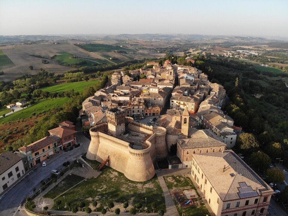
Born here
Currently PhD Student @
Physics of Complex Systems Lab
Advisor: Prof. Matthieu Wyart
Research Interests:
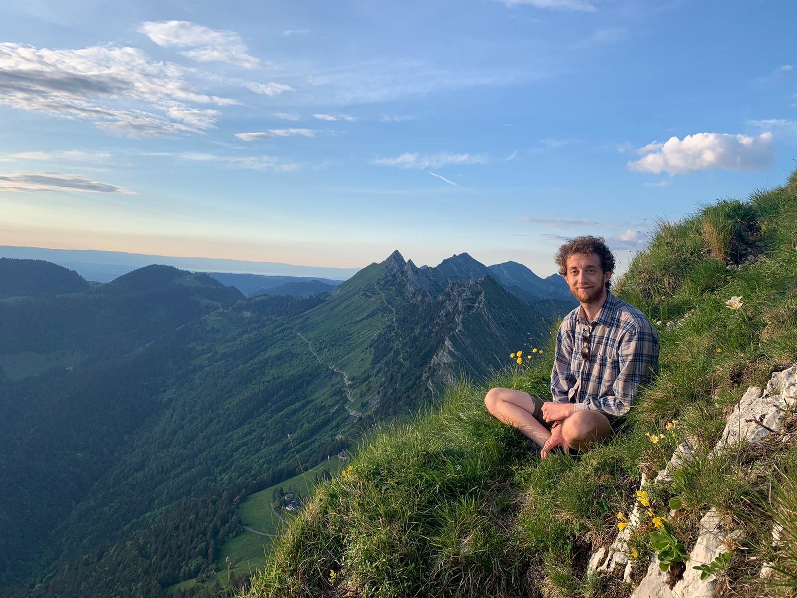
Other interests:
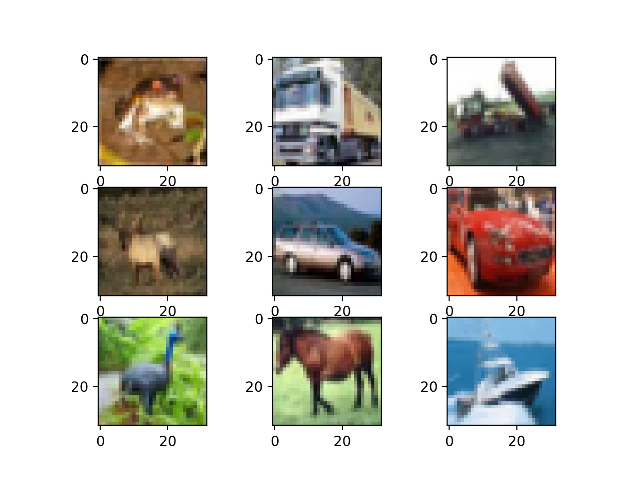
e.g. pixels in the corner are unrelated to the class label
CIFAR10 data-point
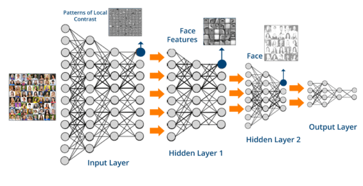
Success of neural nets is often attributed to
(e.g. Mallat, 2016)
Success of neural nets is often attributed to
(e.g. Mallat, 2016)
e.g. pixels in the corner are unrelated to the class label
CIFAR10 data-point
starting from [Jacot et al. 2018] ...
Lazy Regime
weights and NTK are
~constant during learning
Feature Regime
weights and NTK
evolve during learning
Lazy Regime
weights and NTK are
~constant during learning
Cannot learn features of the data
Feature Regime
weights and NTK
evolve during learning
Can possibly learn features and perform compression
starting from [Jacot et al. 2018] ...
Lazy Regime
weights and NTK are
~constant during learning
Cannot learn features of the data
Feature Regime
weights and NTK
evolve during learning
Can possibly learn features and perform compression
starting from [Jacot et al. 2018] ...
Idea... use the evolving NTK to diagnose compression
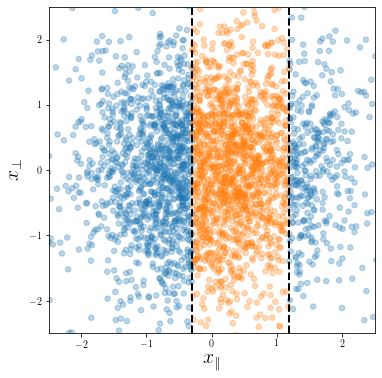
Classification task:
Data-points: \(\vec x = (\vec x_\parallel, \vec x_\bot)\)
Labelling function: \(y(\vec x) = y(\vec x_\parallel) \in \{-1, 1\}\)
Dataset:
Train set size: \(p\)
\(\vec x^\mu \sim \mathcal{N}(0, I_d)\), for \(\mu=1,\dots,p\)
Classification task: \(y(\vec x) = y(\vec x_\parallel) \in \{-1, 1\}\)
Instance for \(d=2\)
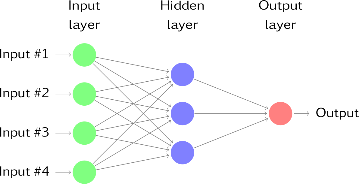
Learning Algo:
◦ Fully connected one-hidden layer NN:
$$f(\vec x) = \frac{1}{h} \sum_{n=1}^h \beta_n \: \sigma \left(\frac{\vec \omega_n \cdot \vec x}{\sqrt{d}} + b_n \right)$$
with \(\sigma(\cdot) = \text{ReLU}(\cdot)\).
◦ Hinge Loss \(l(y, \hat y) = \max(0, 1- y\hat y)\)
◦ Vanilla gradient descent on $$F(\vec x) = \alpha \left(f(\vec x) - f_0(\vec x)\right),$$ where \(f_0\) is the network function at initialization.
Varying \(\alpha\) drives the network dynamics from the feature (small \(\alpha\)) to the lazy (large \(\alpha\)) regime [Chizat et al. 2018].
Fully connected one-hidden layer NN:
$$f(\vec x) = \frac{1}{h} \sum_{n=1}^h \beta_n \: \sigma \left(\frac{\vec \omega_n \cdot \vec x}{\sqrt{d}} + b_n \right)$$
\(\vec x^\mu \sim \mathcal{N}(0, I_d)\), for \(\mu=1,\dots,p\)
Classification task: \(y(\vec x) = y( x_\parallel) \in \{-1, 1\}\)
Compression in the feature regime
weights evolution during training
for a subset of neurons
Compression in the feature regime
weights evolution during training
for a subset of neurons
more tomorrow on Matthieu's lecture
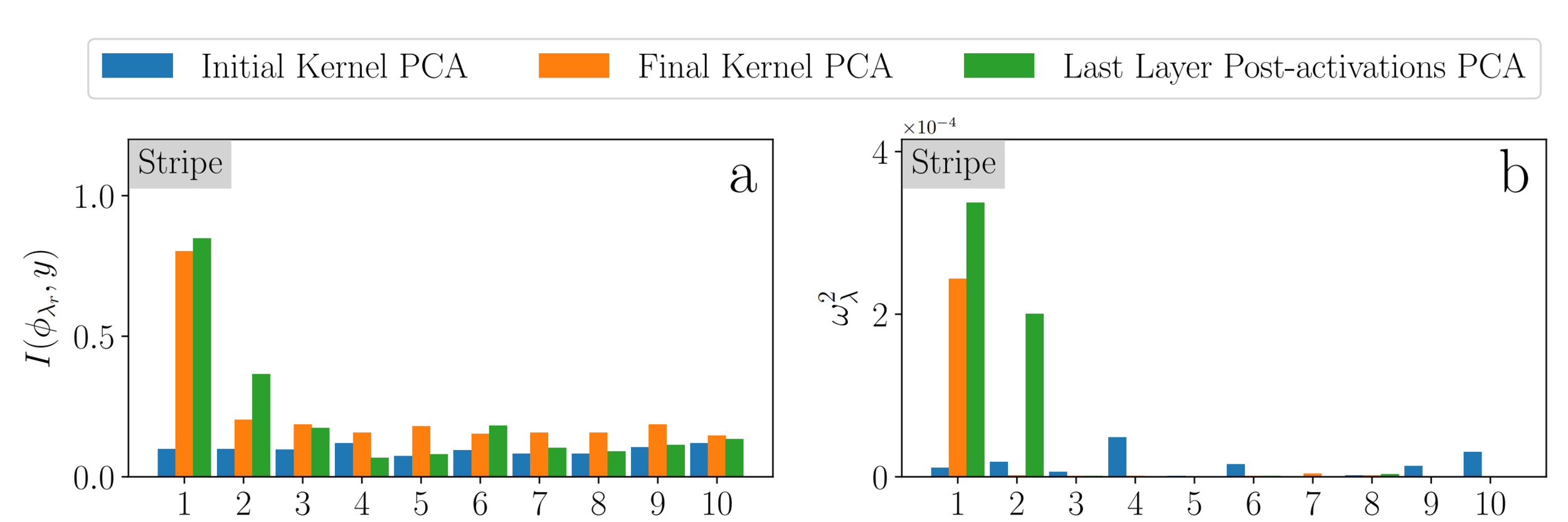
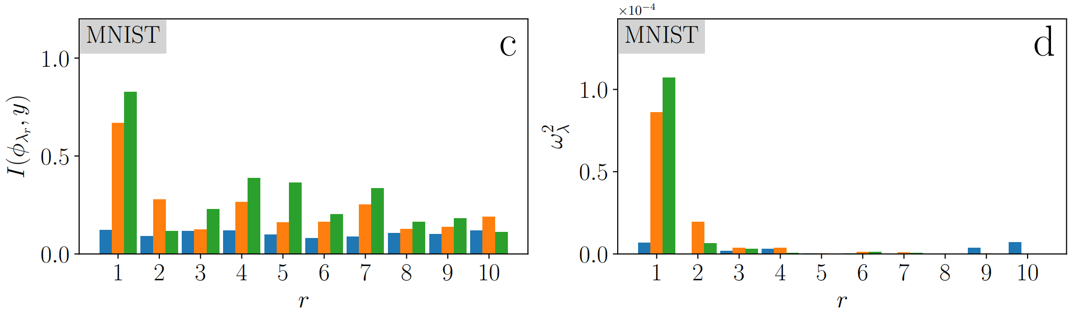
Mutual Information
Projection
We look at the first two
NTK eigenvectors:
(training set size)
The neural tangent kernel [Jacot et al. 2018] is defined as $$\Theta(\vec x^\mu, \vec x^\nu) = \partial_W f(\vec x^\mu) \cdot \partial_W f(\vec x^\nu)$$
where the scalar product runs over all network weights.
Gradient Flow:
$$\partial_t W = \frac{1}{p} \sum_{\mu=1}^p \partial_W f(\vec x^\mu) \, y^\mu \: l'\left(f(\vec x^\mu) \, y^\mu\right),$$
Gradient evolution on functional space:
In general, \(\Theta\) evolves with time.
(training set size)
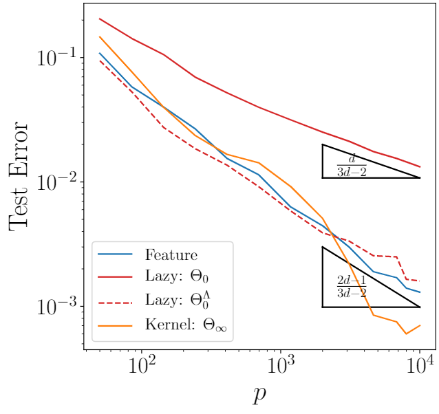
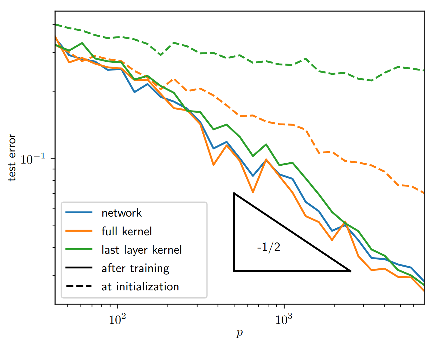
The kernel at the end of learning performs as good as the network itself!
Compression makes the NTK more performant!
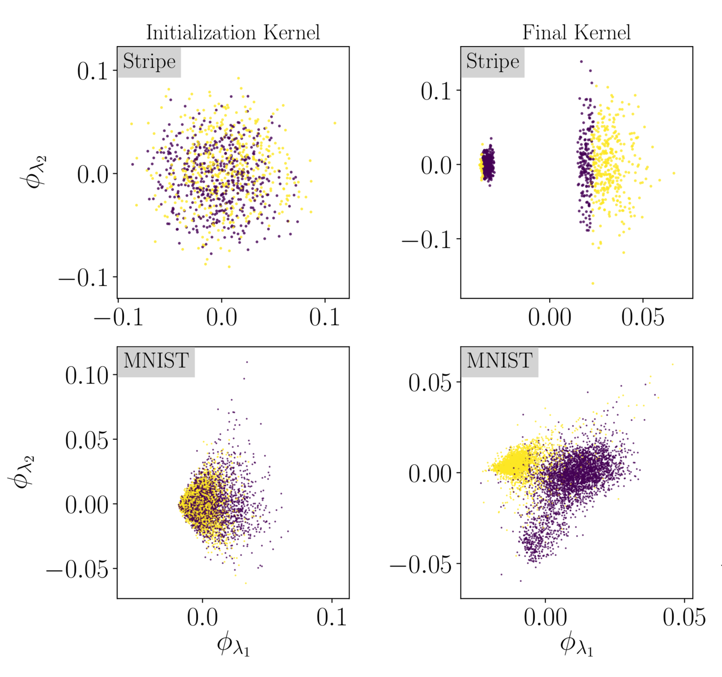
Mutual Information
Projection
Learning Curves
Similarities with Stripe Model
→ hint to compression being key also in MNIST
We look at the first two
NTK eigenvectors values
(color corresponds to class labels)
thank you!
By Leonardo Petrini
Talk for the Statistical Physics and ML Summer Workshop @ Ecole de Physique des Houches, August 2020. Video recording: https://bit.ly/3kQBAYe (from minute 12)


