


Leonardo Petrini
PhD Student @ Physics of Complex Systems Lab, EPFL Lausanne
Leonardo Petrini
joint work with
Francesco Cagnetta, Alessandro Favero, Mario Geiger, Umberto Tomasini, Matthieu Wyart
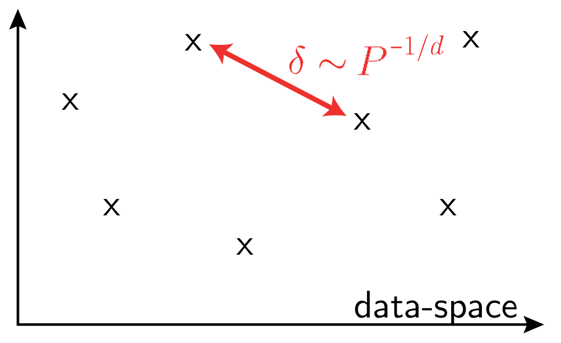
\(P\): training set size
\(d\) data-space dimension
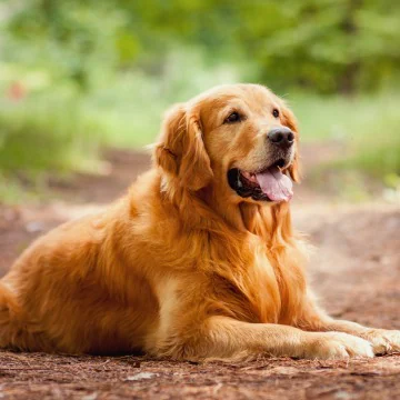
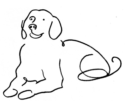
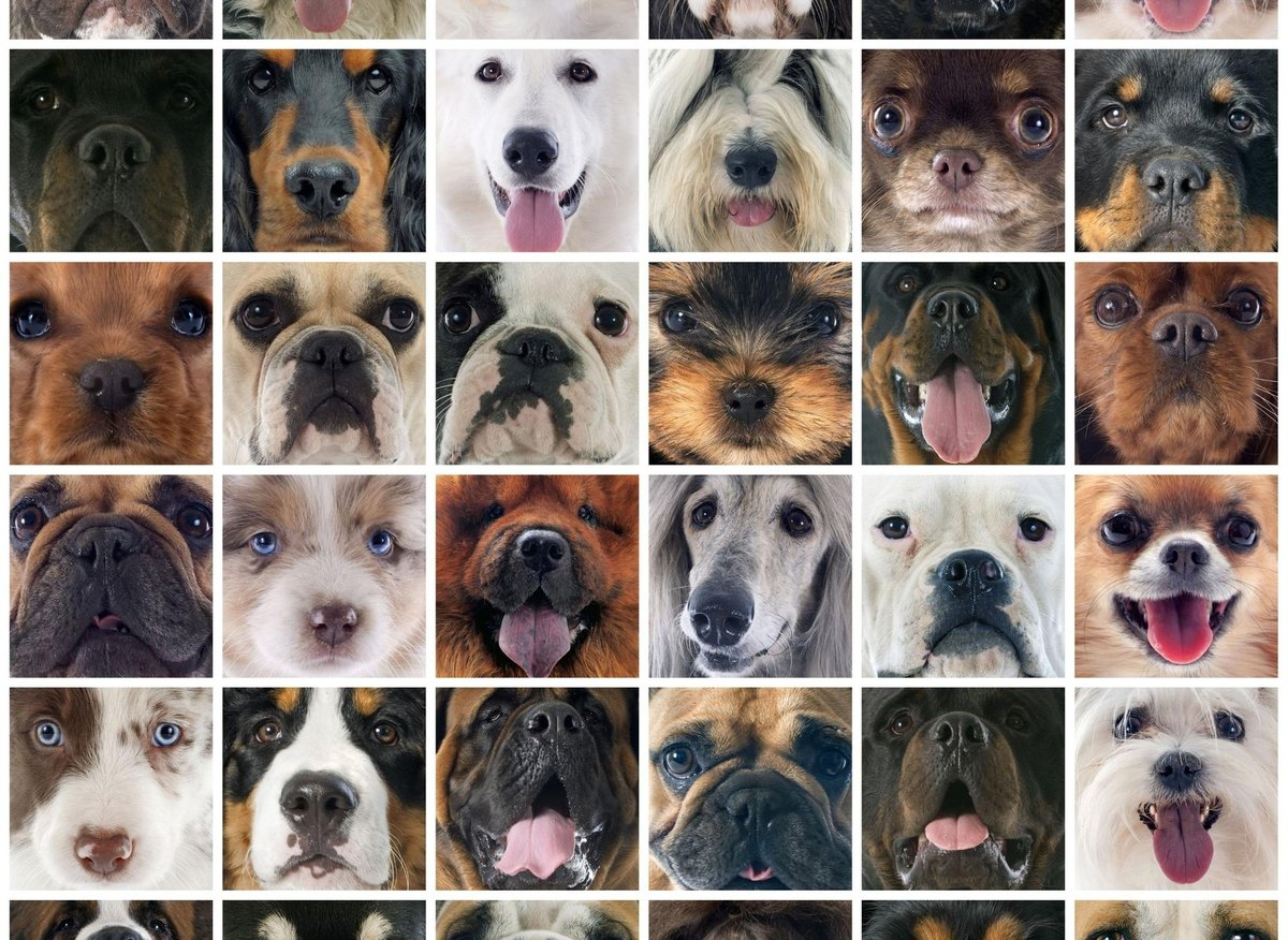
To be learnable, real data must be highly structured
deep net
correct prediction!!
dog
parameters optimized with gradient descent to achieve correct output
e.g. > 90% accuracy for many algorithms and tasks
Language, e.g. ChatGPT
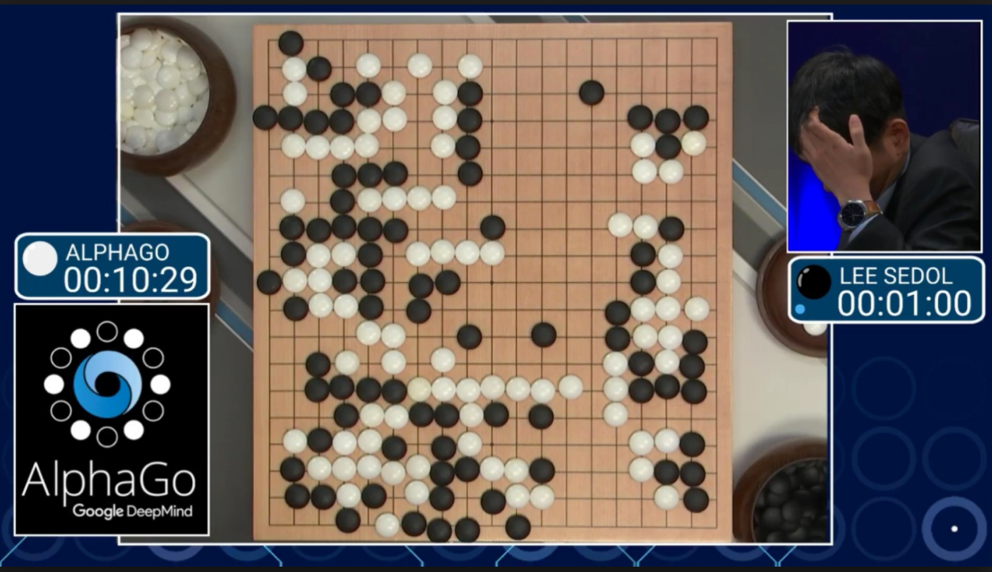
Go-playing
Autonomous cars
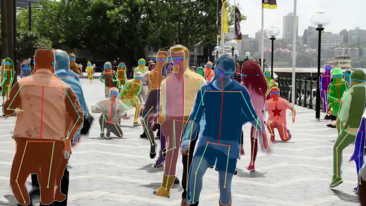
Pose estimation
etc...
Language, e.g. ChatGPT
Go-playing
Autonomous cars
Pose estimation
etc...
\(P\): training set size
\(d\) data-space dimension
Ansuini et al. '19
Recenatesi et al. '19
adapted from Lee et al. '13
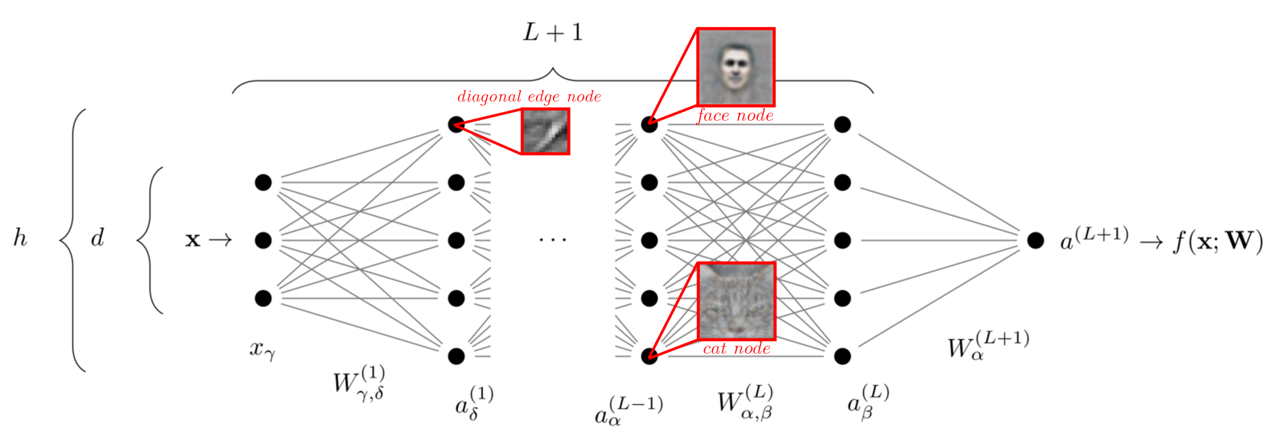
How is dimensionality reduction achieved?
...
dog
face
paws
eyes
nose
mouth
ear
edges
Focus of Part I
Focus of Part II
Mossel '16, Poggio et al. '17, Malach and Shalev-Shwartz '18, '20 Petrini et al '23 (in preparation)
Bruna and Mallat '13, Petrini et al. '21, Tomasini et al. '22
...
dog
face
paws
eyes
nose
mouth
ear
edges
text:
images:
Part I
...
dog
face
paws
eyes
nose
mouth
ear
edges
Previous works:
Poggio et al. '17
Mossel '16, Malach and Shalev-Shwartz '18, '20
Open questions:
Physicist approach:
Introduce a simplified model of data
Q1: Can deep neural networks trained by gradient descent learn hierarchical tasks?
Q2: How many samples do they need?
Previous works:
Physicist approach:
introduce a simplified model of data
Poggio et al. '17
Mossel '16, Malach and Shalev-Shwartz '18, '20
adapted from Lee et al. '13
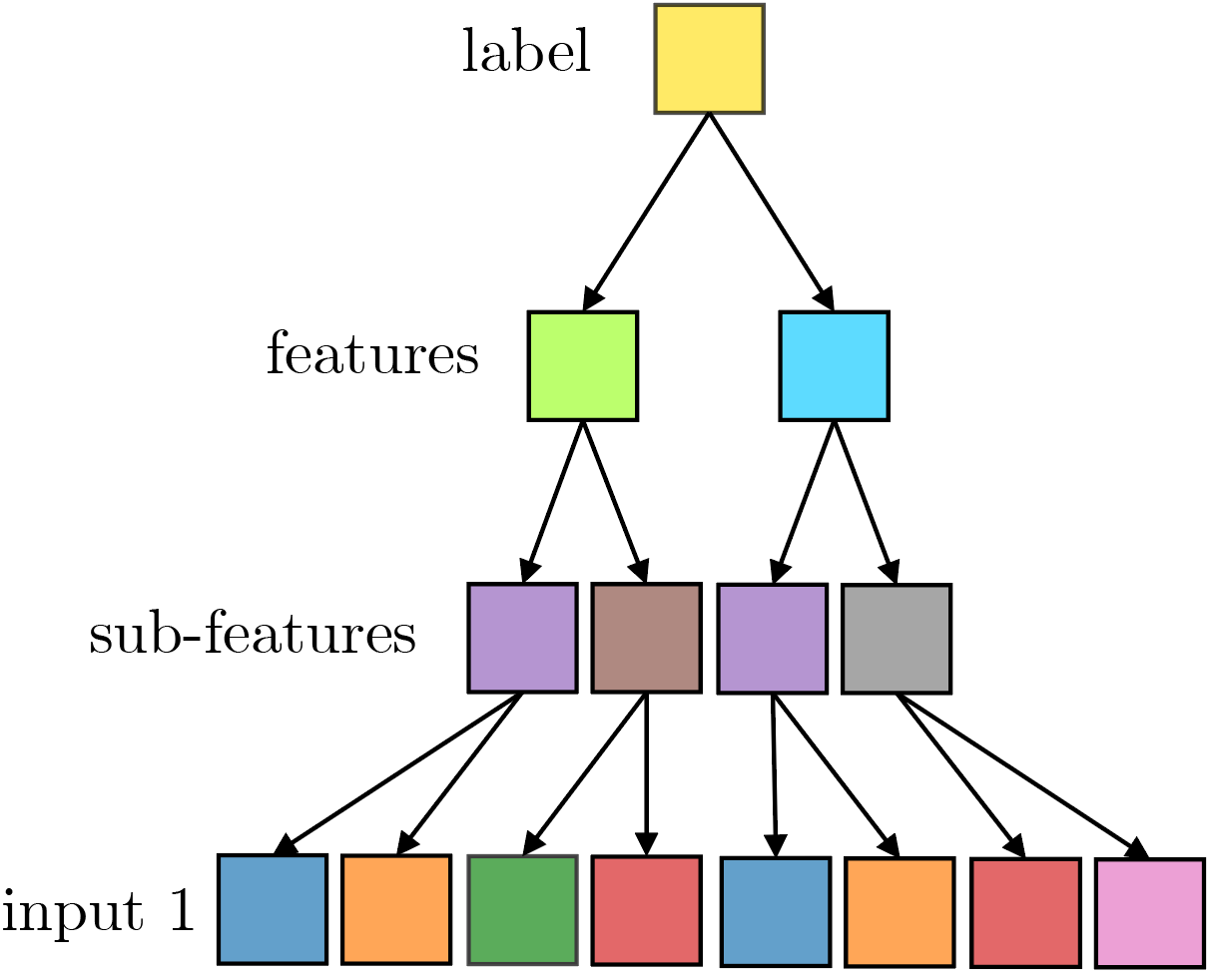
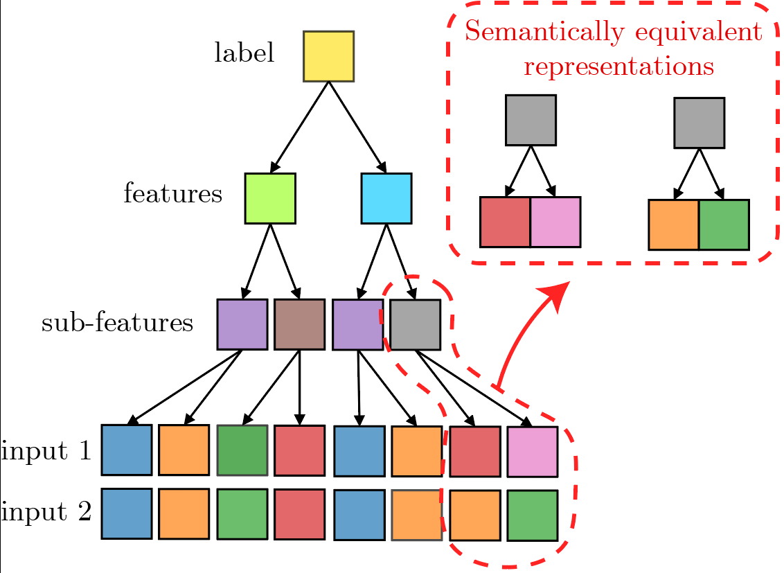
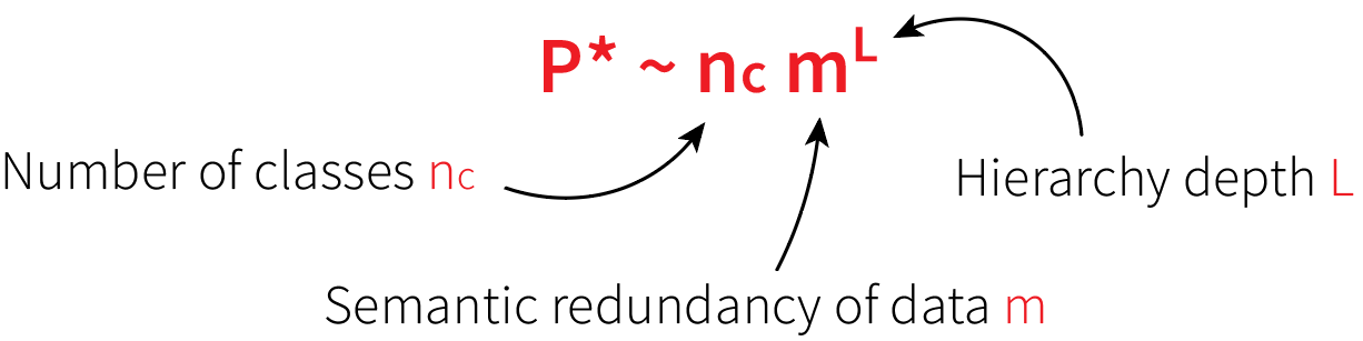
Propose generative model of hierarhical data and study sample complexity of neural networks.
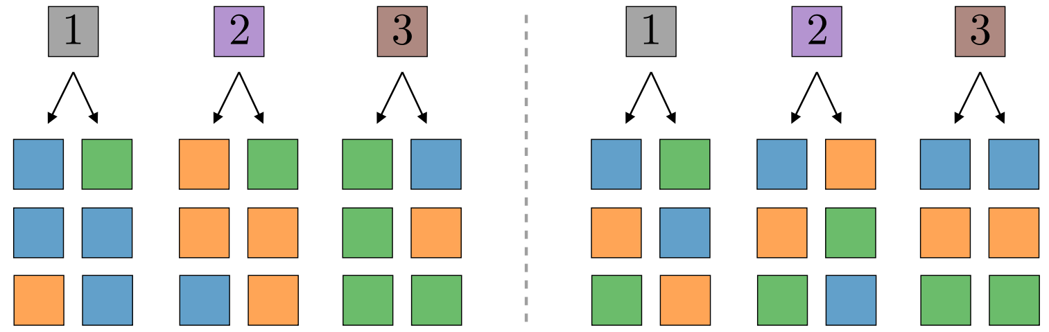
2) Finite vocabulary:
4) Random (frozen) rules:
- The \(m\) possible strings of a class are chosen uniformly at random among the \(v^s\) possible ones;
- Same for features, etc...
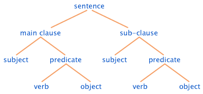
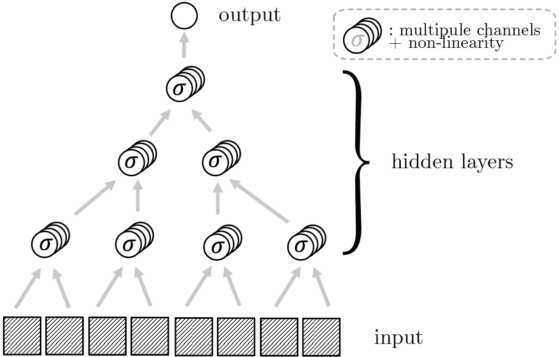
1) Hierarchy:
3) Degeneracy:
To generate data, for a given choice of \((v, n_c, m, L, s)\):
At every level, semantically equivalent representations exist.
How many points do neural networks need to learn these tasks?
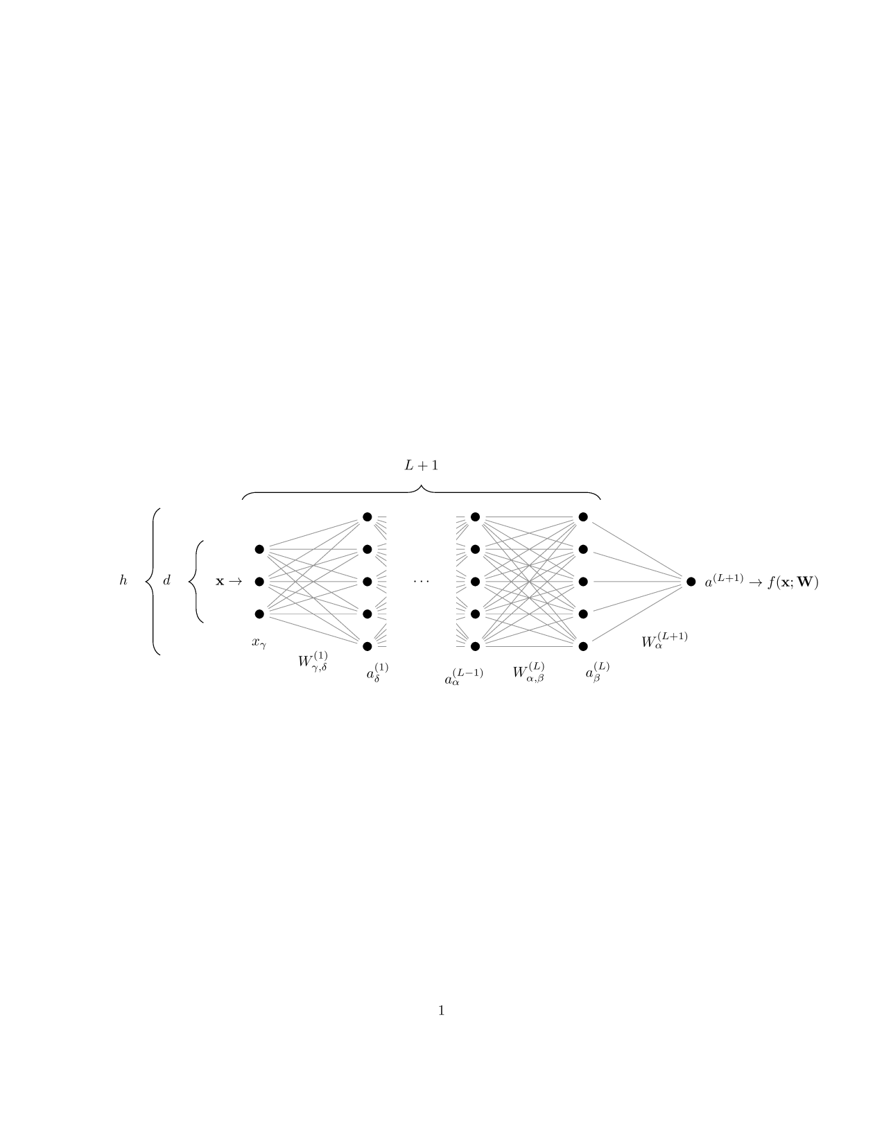
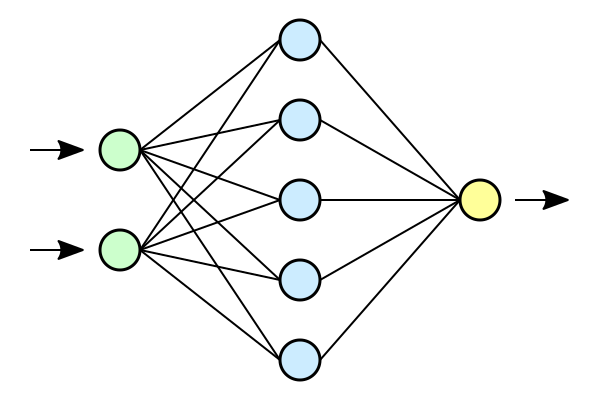
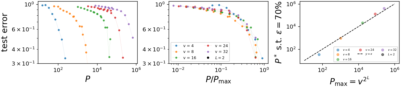
Training a one-hidden-layer fully-connected neural network
with gradient descent to fit a training set of size \(P\).
original
rescaled \(x-\)axis
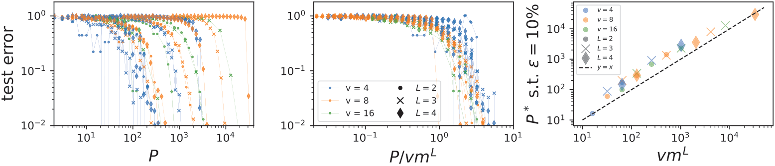
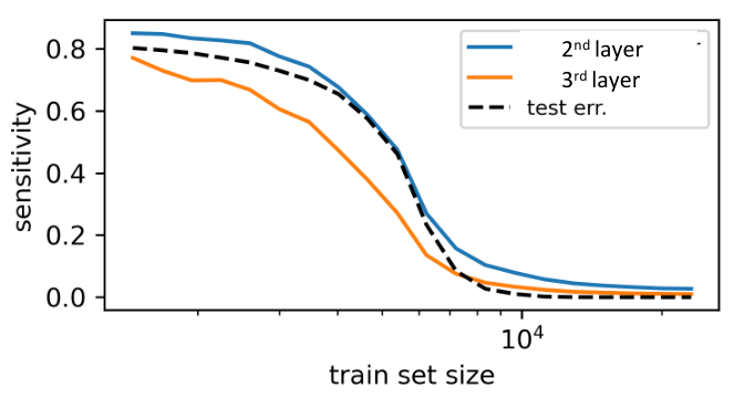
Training a deep convolutional neural networks with \(L\)
hidden layers on a training set of size \(P\).
original
rescaled \(x-\)axis
Training a deep convolutional neural networks with \(L\)
hidden layers on a training set of size \(P\).
original
rescaled \(x-\)axis
Can we understand DNNs success?
Are they learning the structure of the data?
How is semantic invariance learned?
= sample complexity of DNNs!!
At each level of the hierarchy, correlations exist between higher and lower level features.
Rules are chosen uniformly
at random:
correlated rule (likely)
uncorrelated rule (unlikely)
\(\alpha\) : class
\(\mu\) : low-lev. feature
\(j\) : input location
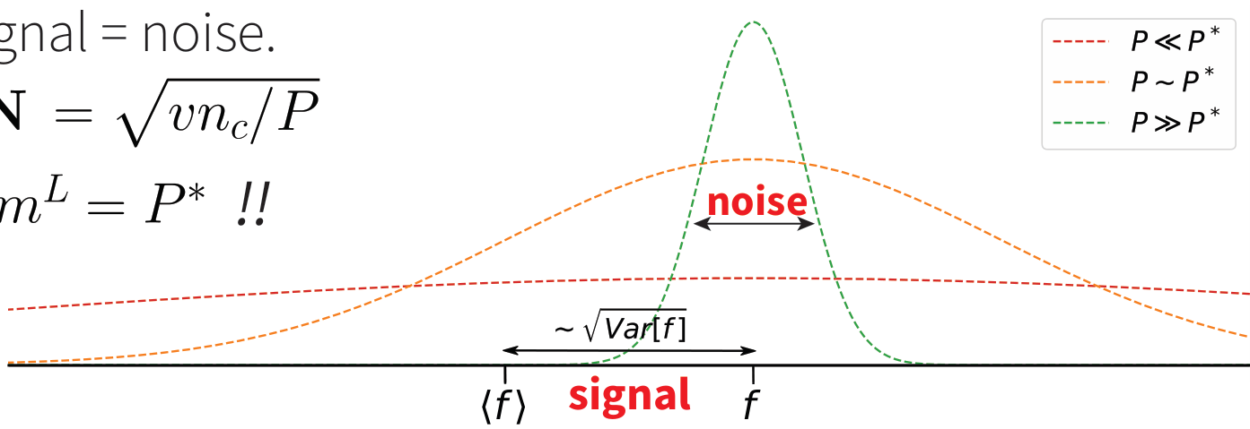
These correlations (signal) are given by the variance of $$f_j(\alpha | \mu ) := \mathbb{P}\{x\in\alpha| x_j = \mu\}.$$
For \(P < P_\text{max}\) , \(f\)'s are estimated from empirical counterpart (sampling noise).
Learning is possible starting from signal = noise.
We compute \(\mathbf{S}\sim \sqrt{v/m^L}\), \(\mathbf{N}\sim \sqrt{vn_c/P}\):
observe
At each level of the hierarchy, correlations exist between higher and lower level features.
Rules are chosen uniformly
at random:
correlated rule (likely)
uncorrelated rule (unlikely)
\(\alpha\) : class
\(\mu\) : low-lev. feature
\(j\) : input location
These correlations (signal) are given by the variance of $$f_j(\alpha | \mu ) := \mathbb{P}\{x\in\alpha| x_j = \mu\}.$$
For \(P < P_\text{max}\) , \(f\)'s are estimated from empirical counterpart (sampling noise).
Learning is possible starting from signal = noise.
We compute \(\mathbf{S}\sim \sqrt{v/m^L}\), \(\mathbf{N}\sim \sqrt{vn_c/P}\):
What are correlations used for?
observe
At each level of the hierarchy, correlations exist between higher and lower level features.
Rules are chosen uniformly
at random:
correlated rule (likely)
uncorrelated rule (unlikely)
\(\alpha\) : class
\(\mu\) : low-lev. feature
\(j\) : input location
These correlations (signal) are given by the variance of $$f_j(\alpha | \mu ) := \mathbb{P}\{x\in\alpha| x_j = \mu\}.$$
For \(P < P_\text{max}\) , \(f\)'s are estimated from empirical counterpart (sampling noise).
Learning is possible starting from signal = noise.
We compute \(\mathbf{S}\sim \sqrt{v/m^L}\), \(\mathbf{N}\sim \sqrt{vn_c/P}\):
observe
On hierarchical tasks:
Focus of Part I
Focus of Part II
Mossel '16, Poggio et al. '17, Malach and Shalev-Shwartz '18, '20 Petrini et al '23 (in preparation)
Bruna and Mallat '13, Ansuini et al. '19, Recenatesi et al. '19 Petrini et al. '21, Tomasini et al. '22
...
dog
face
paws
eyes
nose
mouth
ear
edges
text:
images:
Focus of Part I
Focus of Part II
Mossel '16, Poggio et al. '17, Malach and Shalev-Shwartz '18, '20 Petrini et al '23 (in preparation)
Bruna and Mallat '13, Ansuini et al. '19, Recenatesi et al. '19 Petrini et al. '21, Tomasini et al. '22
...
dog
face
paws
eyes
nose
mouth
ear
edges
text:
images:
Part II
Is it true or not?
Can we test it?
Bruna and Mallat '13, Mallat '16
Plan:
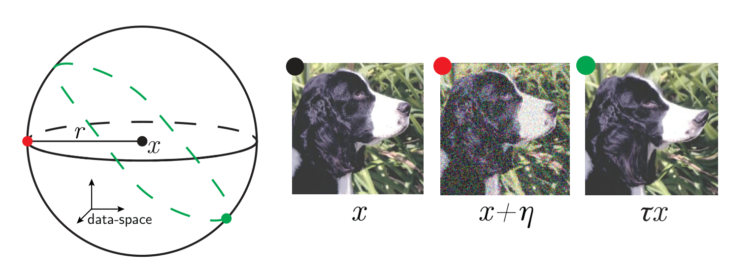
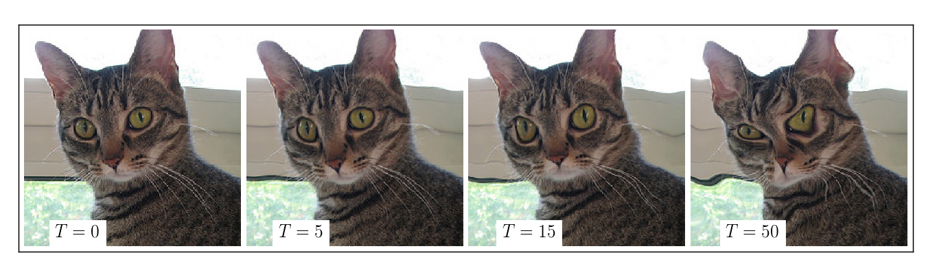
more deformed
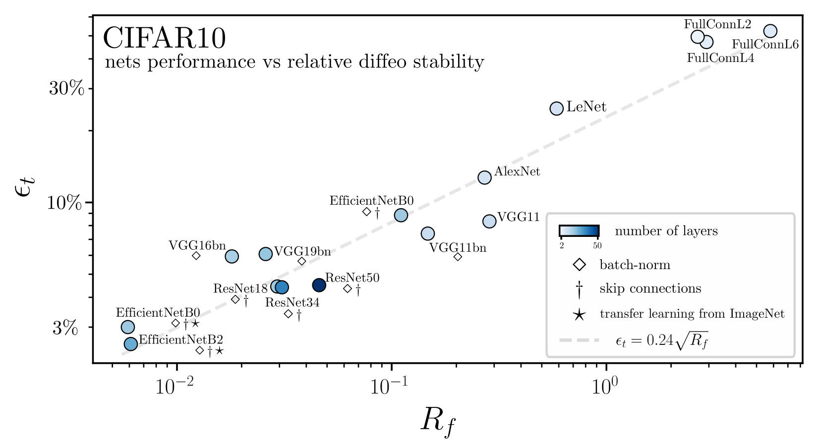
Invariance measure: relative stability
(normalized such that is =1 if no diffeo stability)
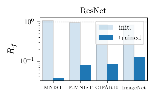
Results:
Deep nets learn to become stable to diffeomosphisms!
Relationship with performance?
see Tomasini et al. '22
Thank you!
Pt. 1
Pt. 2
By Leonardo Petrini
We aim to answer the fundamental question of how deep learning algorithms achieve remarkable success in processing high-dimensional data, such as images and text, while overcoming the curse of dimensionality. This curse makes it challenging to efficiently sample data and can result in a sample complexity, which is the number of data points needed to learn a task, scaling exponentially with the space dimension in generic settings. Our investigation centers on the idea that to be learnable, real-world data must be highly structured. We explore two aspects of this idea: (i) the hierarchical nature of data, where higher-level features are a composition of lower-level features, such as how a face is made up of eyes, nose, mouth, etc., (ii) the irrelevance of the exact spatial location of such features. Following this idea, we investigate the hypothesis that deep learning is successful because it constructs useful hierarchical representations of data that exploit its structure (i) while being insensitive to aspects irrelevant for the task at hand (ii).


