


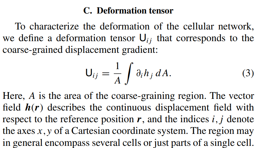


Leonardo Petrini
PhD Student @ Physics of Complex Systems Lab, EPFL Lausanne
PCSL internal group meeting
October 7, 2021
vs.
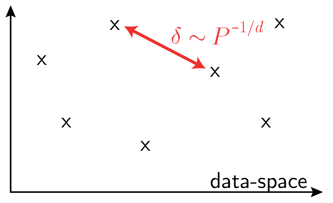
\(P\): training set size
\(d\) data-space dimension
Hypothesis: images can be classified because the task is invariant to smooth deformations of small magnitude and CNNs exploit such invariance with training.
Bruna and Mallat (2013) Mallat (2016)
...
Is it true or not?
Can we test it?
"Hypothesis" means, informally, that
\(\|f(x) - f(\tau x)\|^2\) is small if the deformation is small.
\(x\) : data-point
\(\tau\) : smooth deformation
\(f\) : network function
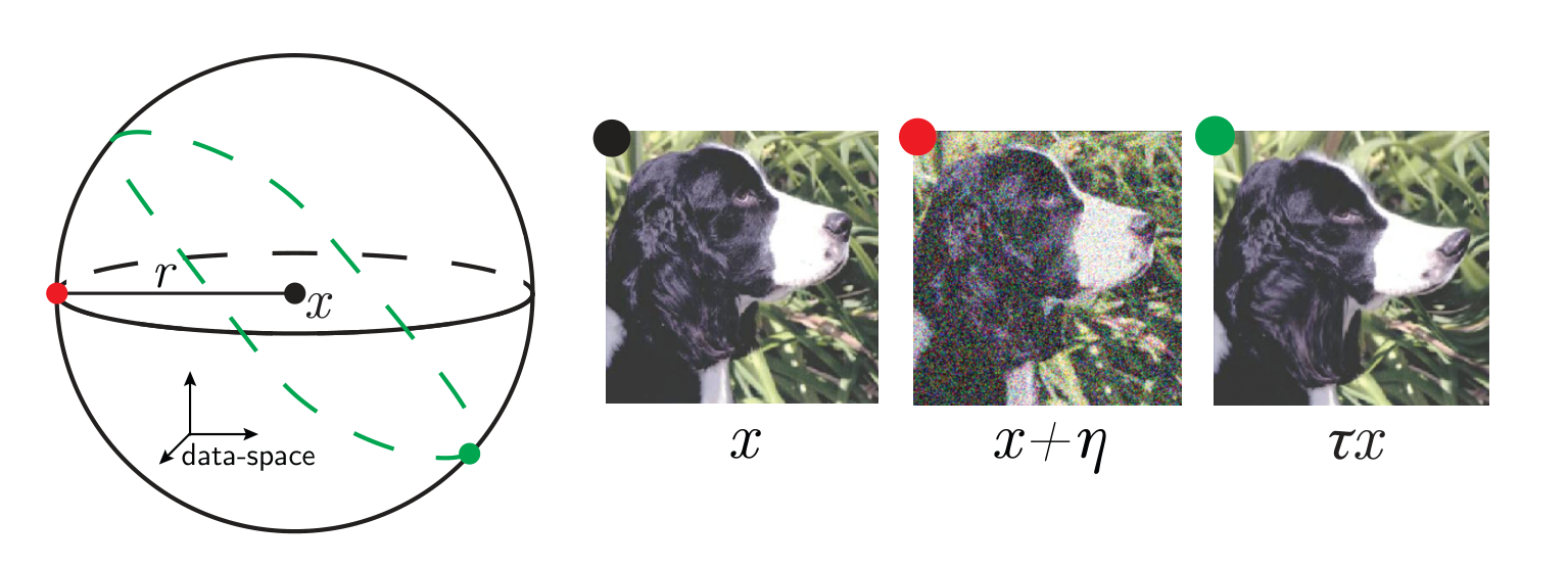
Yes! We can
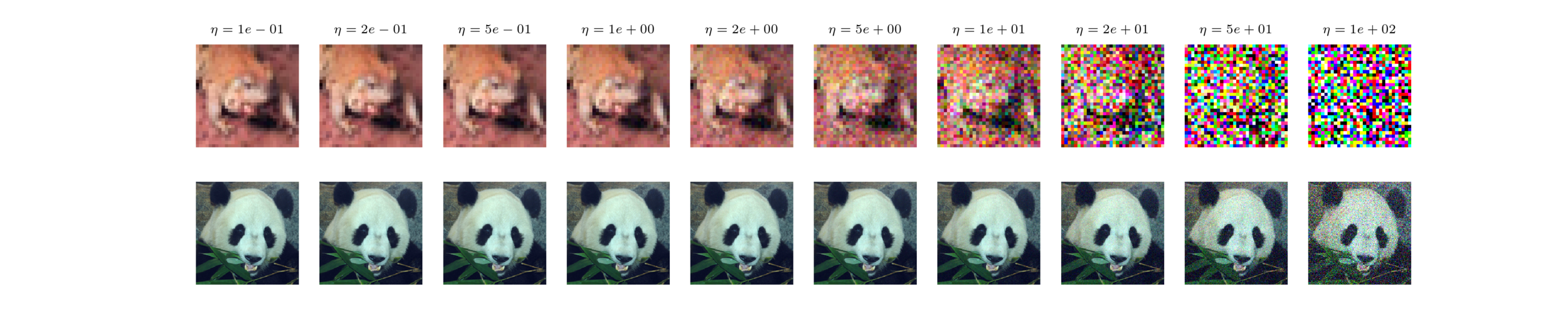
\(x\) input image
\(\tau\) smooth deformation
\(\eta\) isotropic noise with \(\|\eta\| = \langle\|\tau x - x\|\rangle\)
\(f\) network function
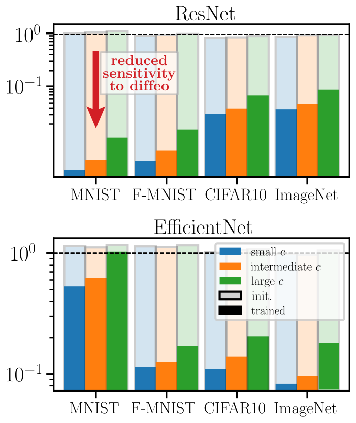
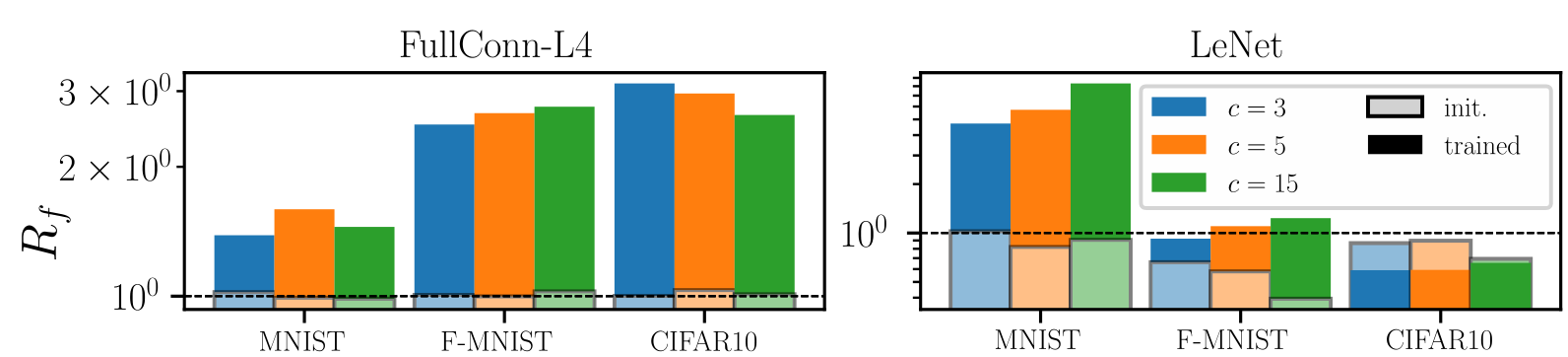
Goal: quantify how a deep net learns to become less sensitive
to diffeomorphisms than to generic data transformations
$$R_f = \frac{\langle \|f(\tau x) - f(x)\|^2\rangle_{x, \tau}}{\langle \|f(x + \eta) - f(x)\|^2\rangle_{x, \eta}}$$
Relative stability:
$$R_f = \frac{\langle \|f(\tau x) - f(x)\|^2\rangle_{x, \tau}}{\langle \|f(x + \eta) - f(x)\|^2\rangle_{x, \eta}}$$
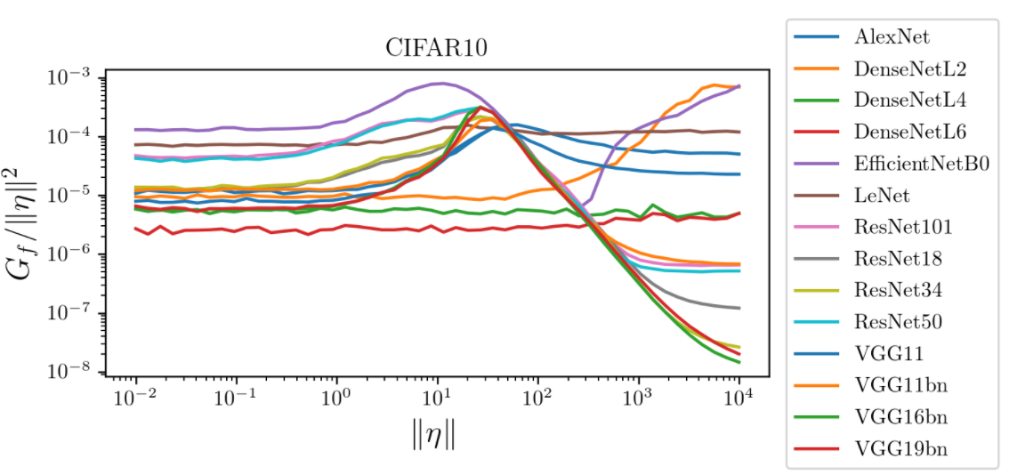
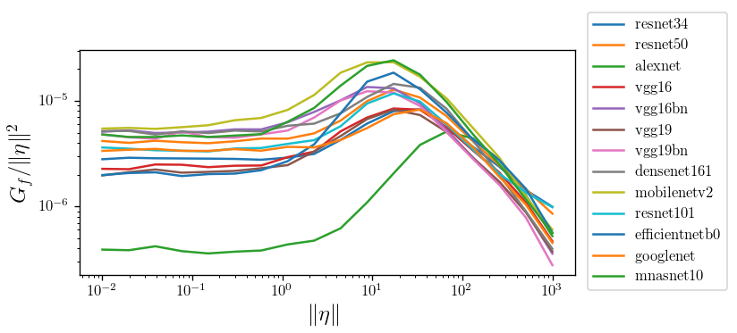
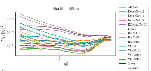
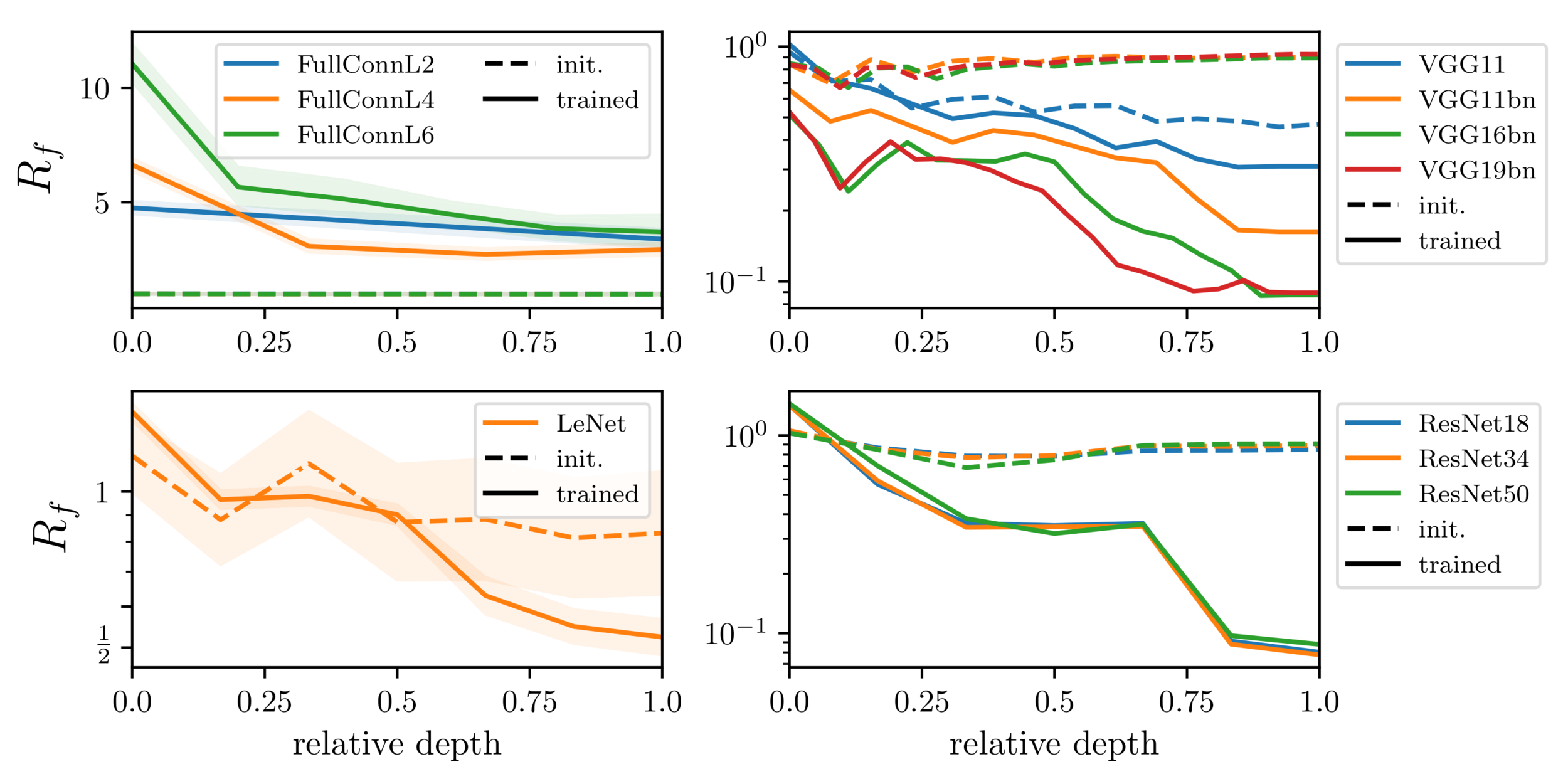
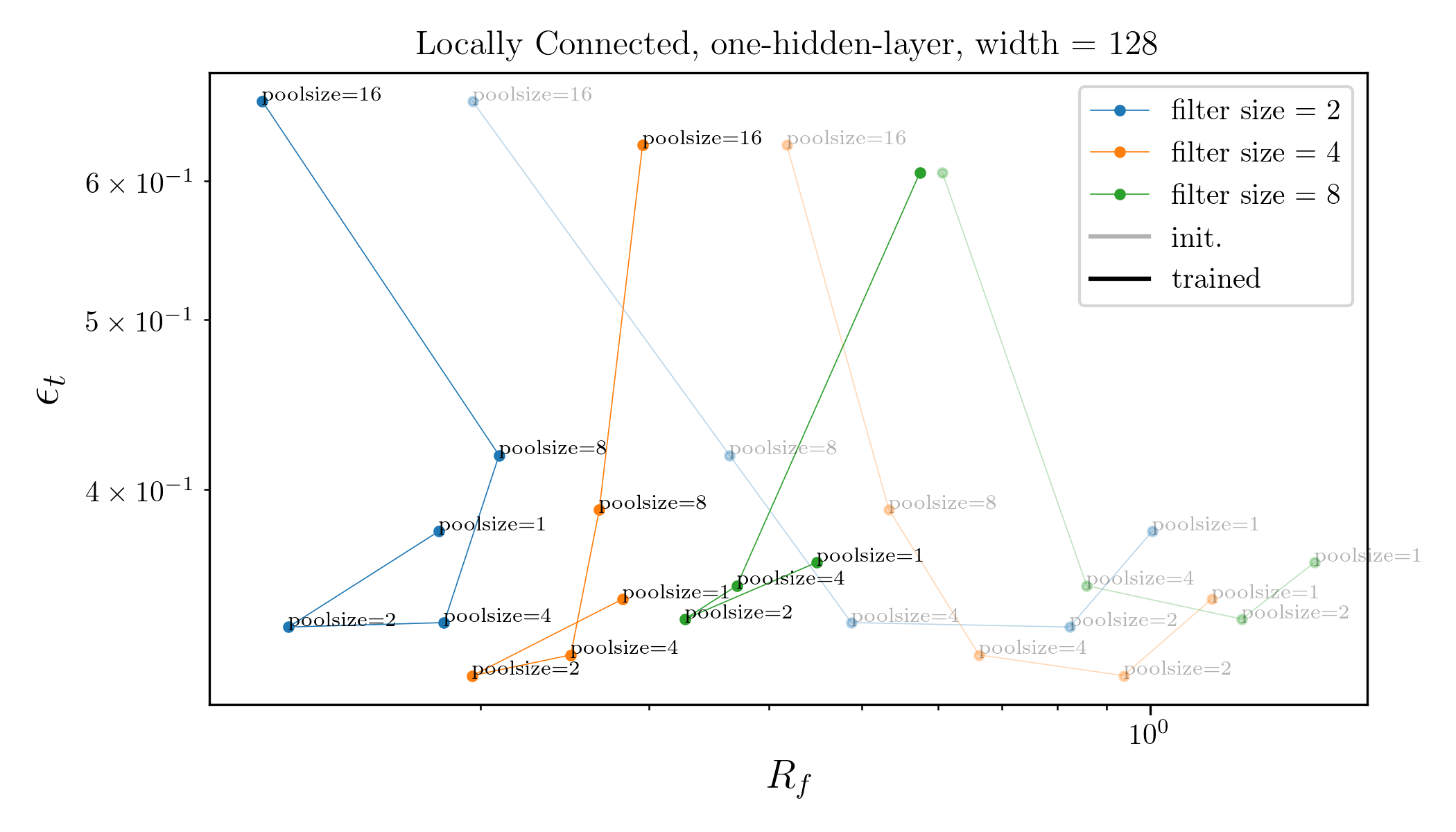
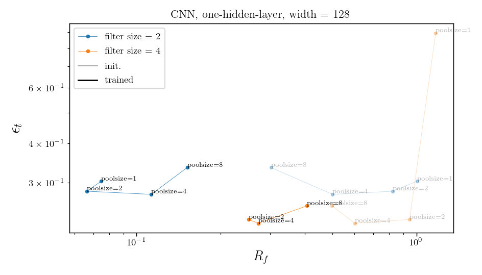
Results:
Deep nets learn to become stable to diffeomosphisms!
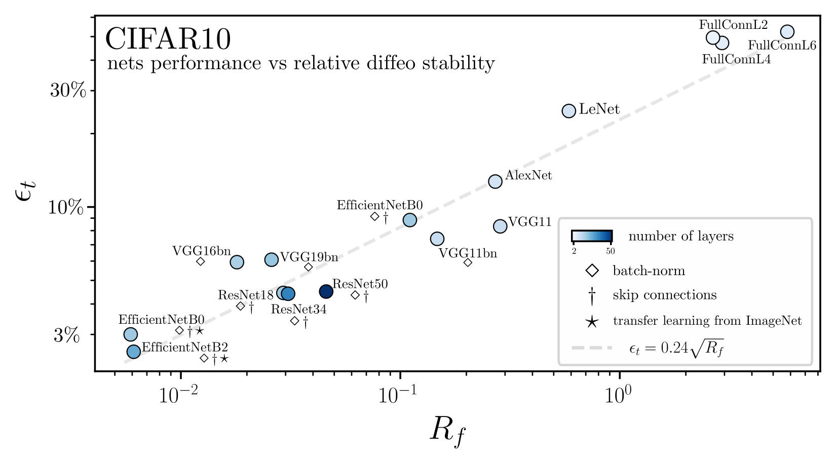
Is there a relation with performance?
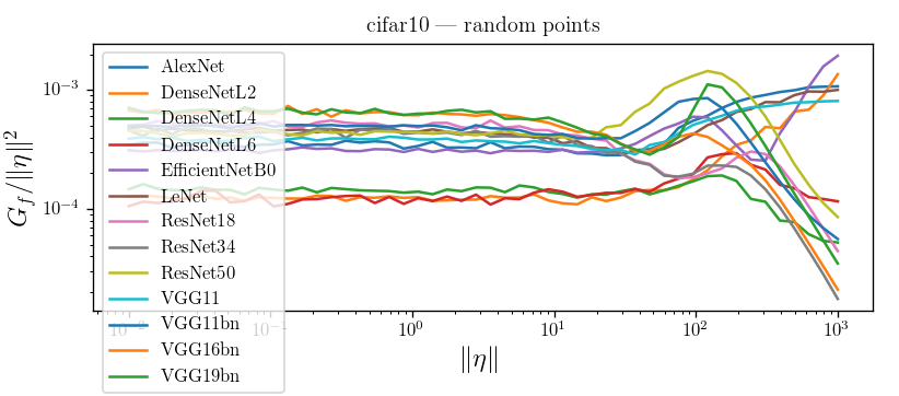
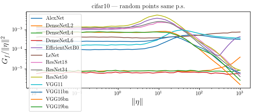
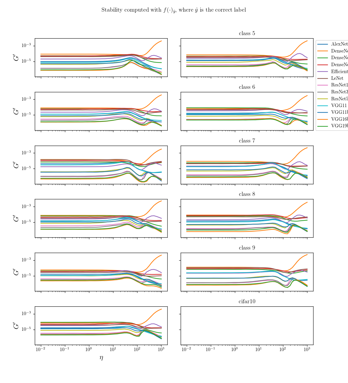
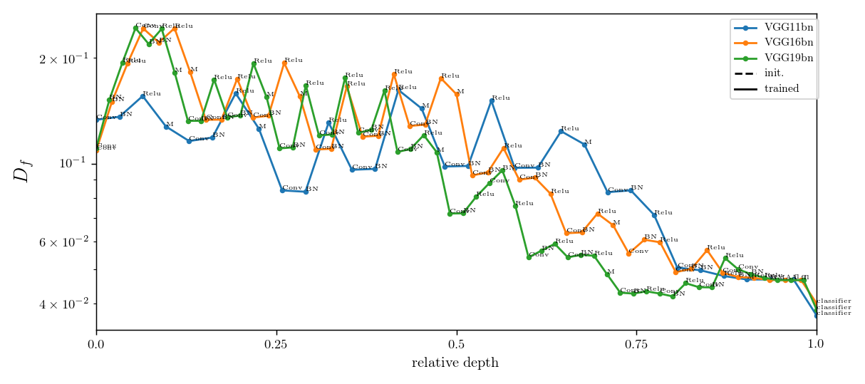
What's the shape of \(D_f\) and \(G_f\) as a function of \(r = \|\eta\|\)?
i.e. how does the predictor look like while moving away from datapoints?
diffeo stability
additive noise stability
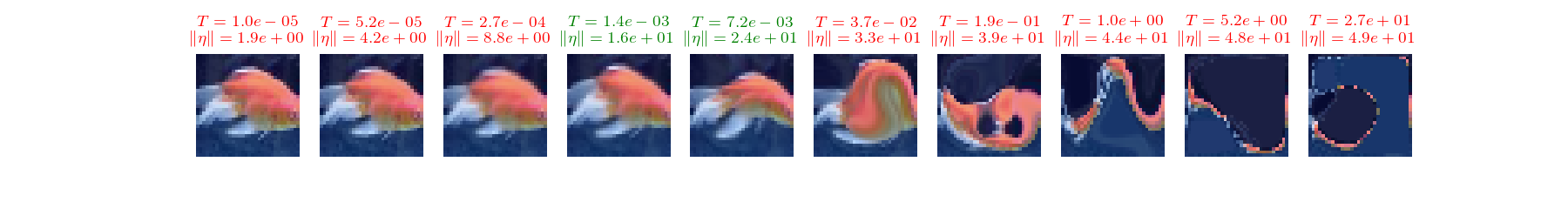
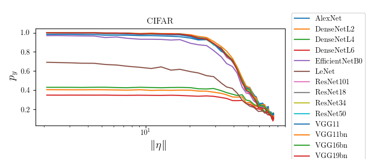
Recall:
Linear regime
bump
Linear regime
bump
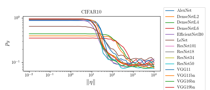
Recall: to train a net with cross-entropy loss we apply a softmax to the output
where \(\hat p_i\) can be interpreted as probability that the network assigns to \(i\) being the correct class
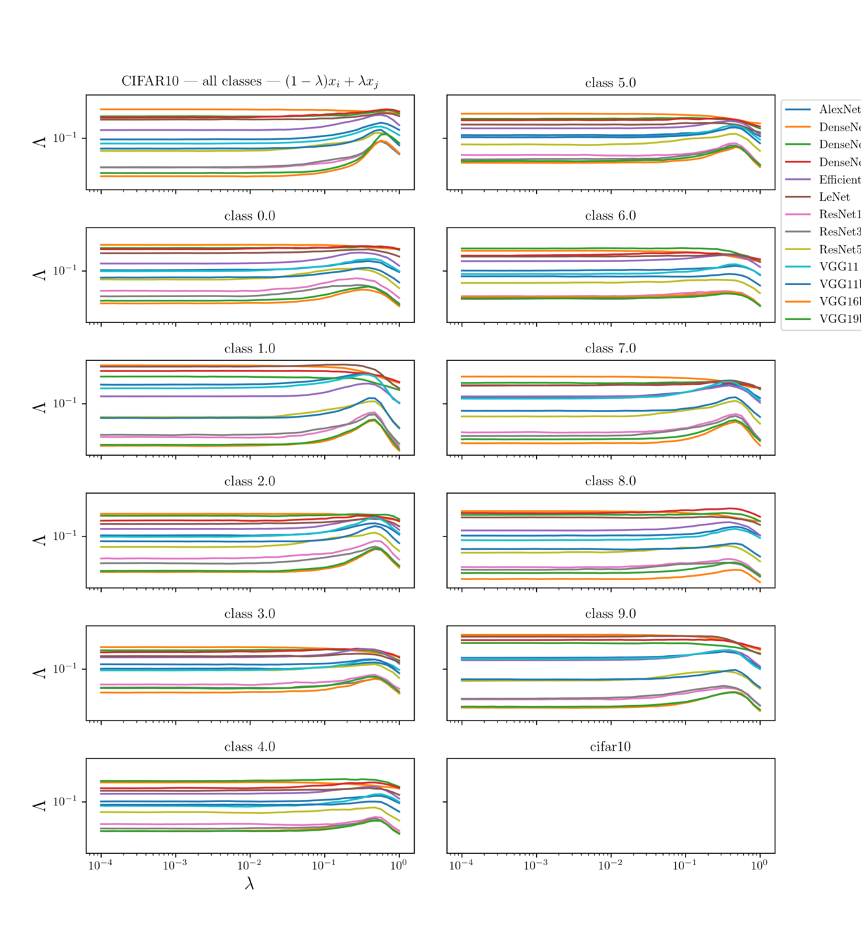
Bump corresponds to the regime in which nets start misclassifying!
Visually, the position of the bump makes sense for CIFAR10, not much for ImageNet
CIFAR10:
ImageNet:
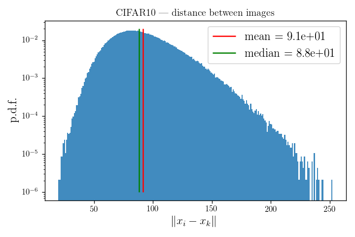
where \(\eta_z\) is pointing in the direction of another datapoint \(z\)
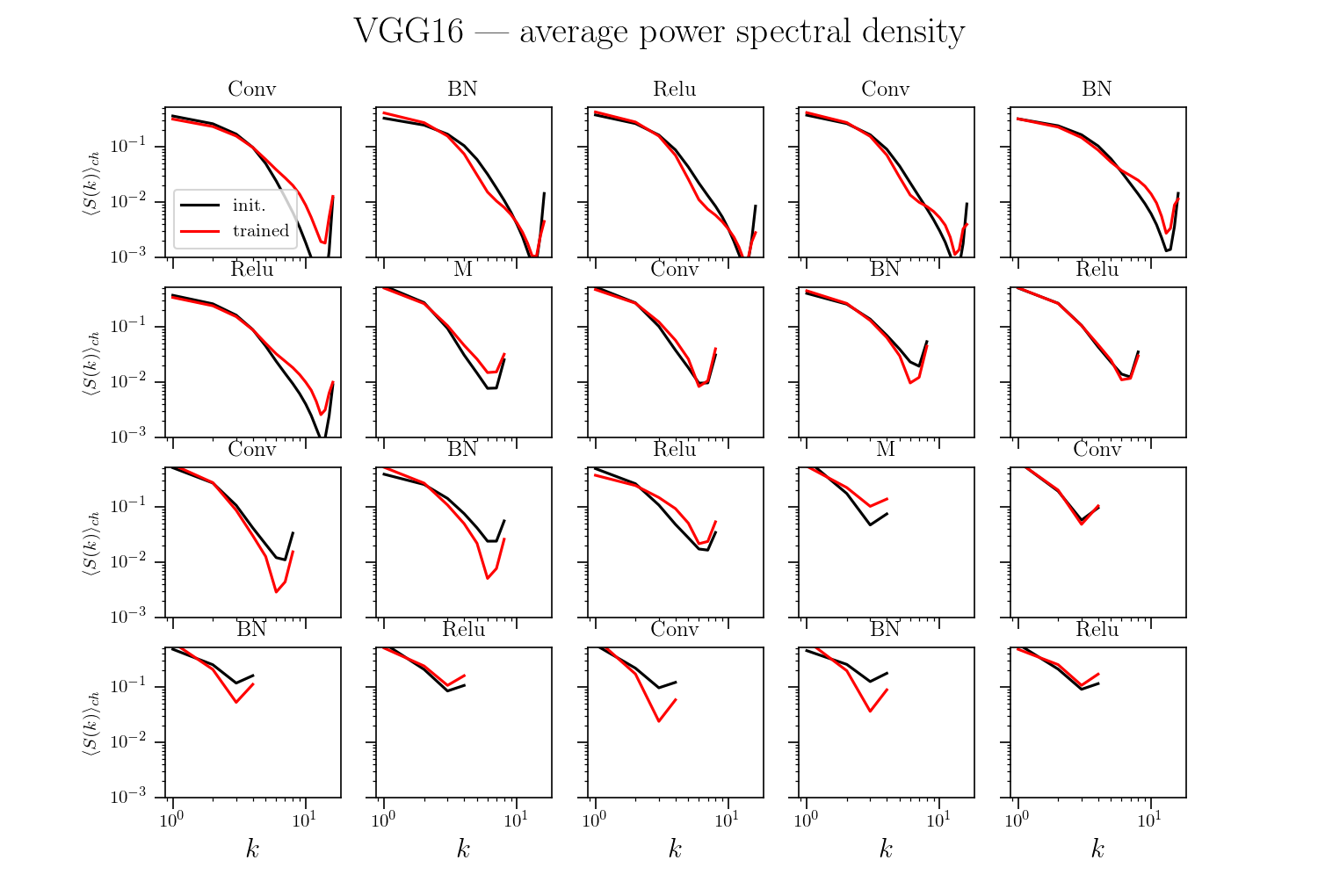
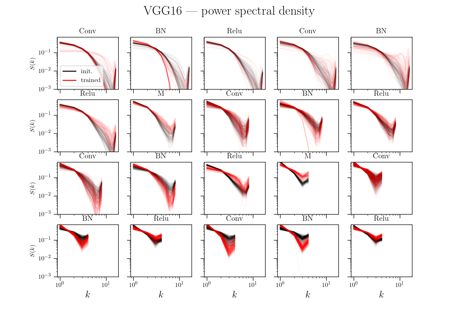
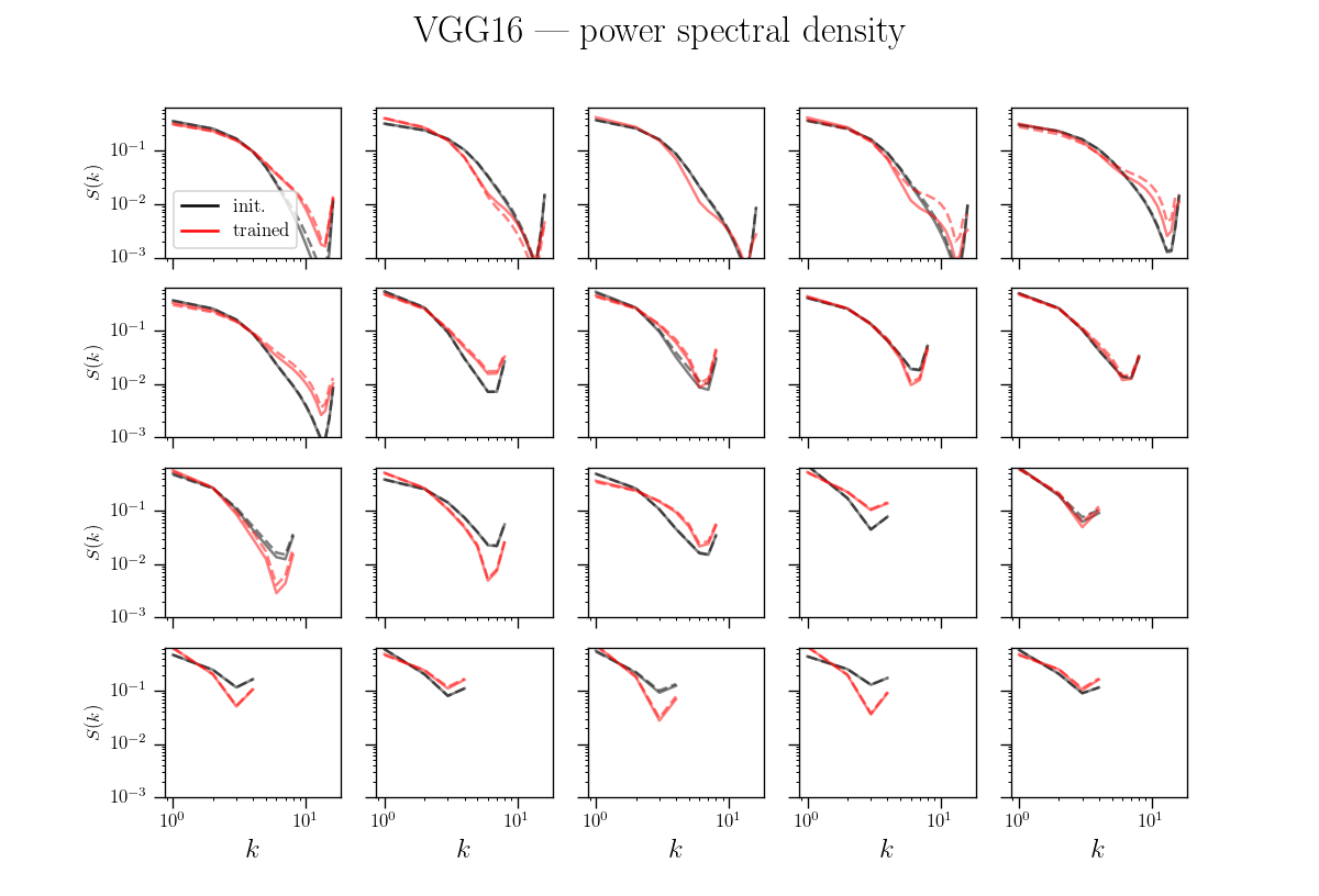
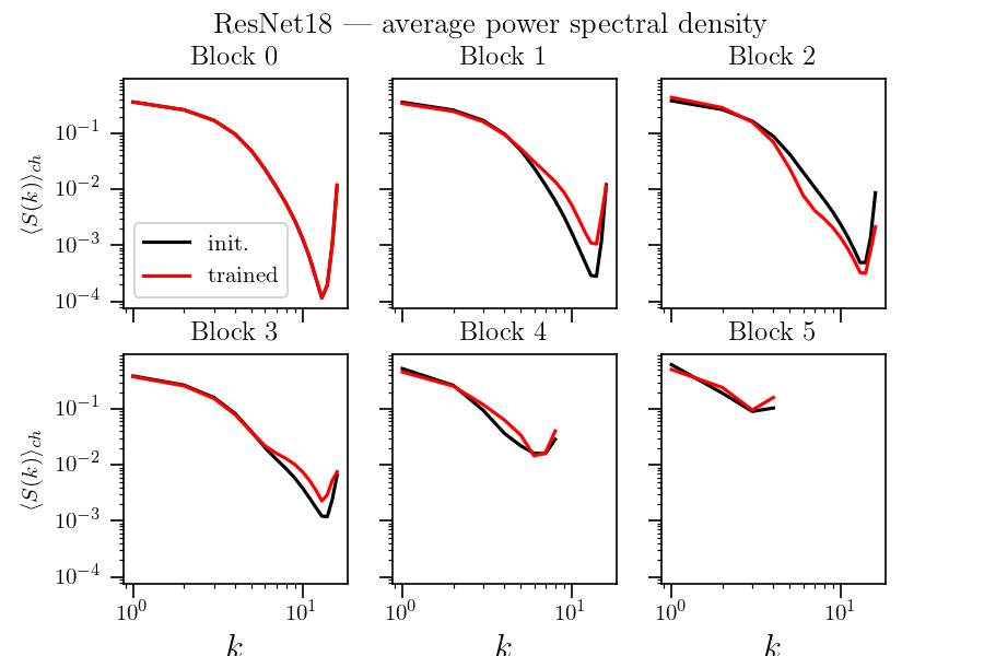
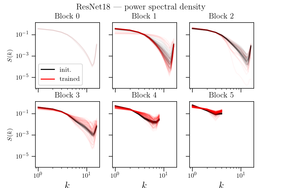
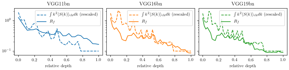
Hypothesis: nets become relatively stable by making filters low-pass with training.
If hyp. is true, the activations power spectrum should become more low-frequency after training.
We test it...
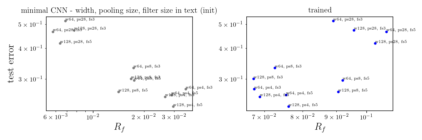
Simple models show a different phenomenology than SOTA nets
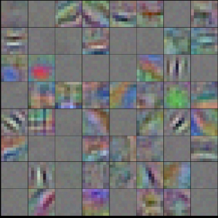
Here a net trained with 9x9 filters seems to get to Gabor filters
Usually, 3x3 filters are used though.
Here,
for each channel
Same as previous slide plus (in dashed) the power spectral density when normalizing power spectra before averaging over channels
Hypothesis: nets become relatively stable by making filters low-pass with training.
back to our hypothesis...
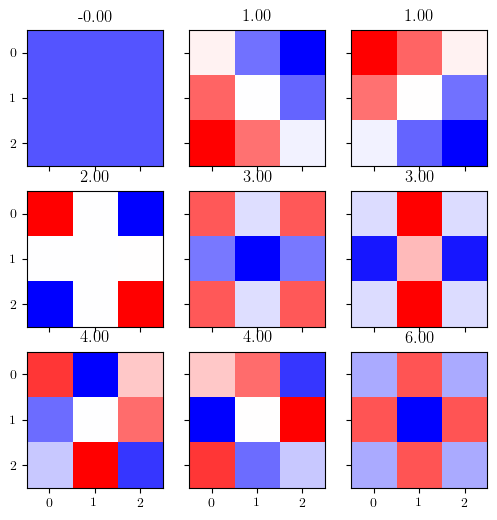
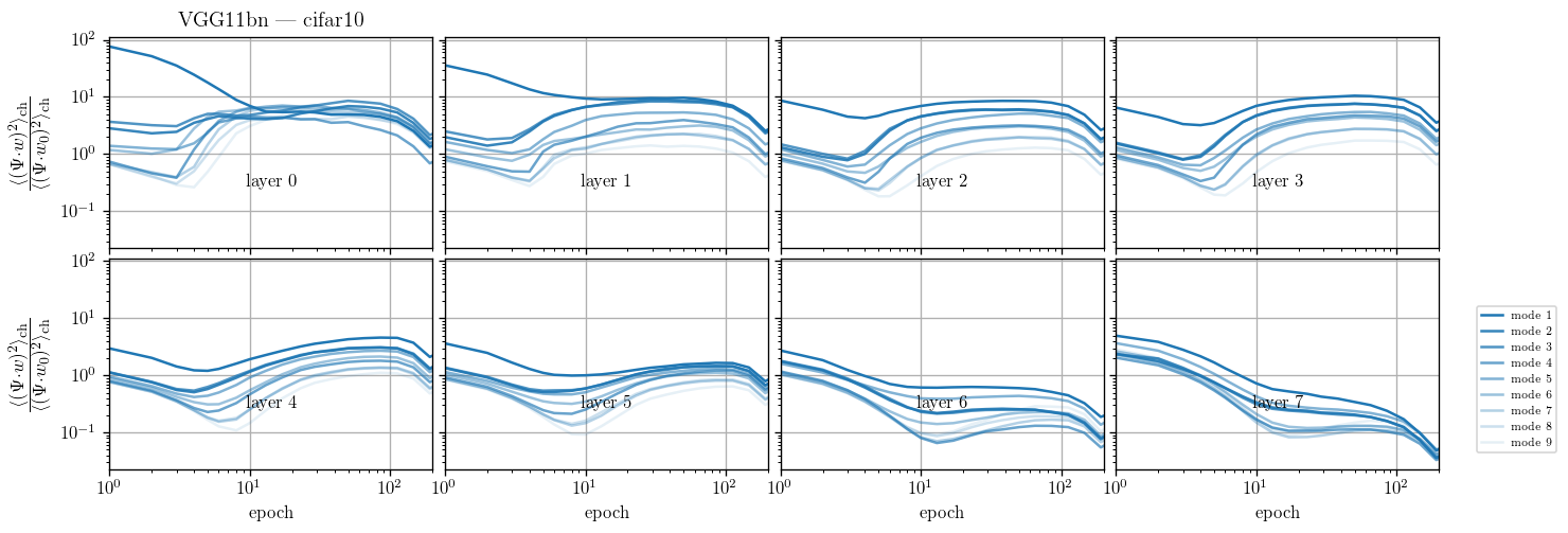
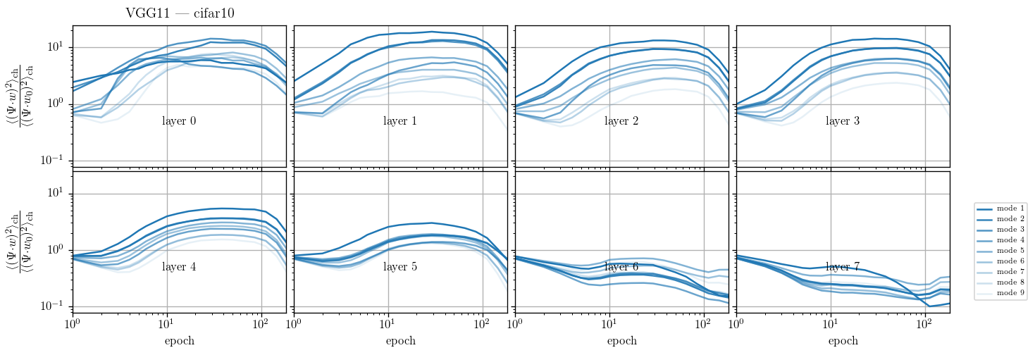
We take a basis that is the eigenvectors of the Laplacian on the 3x3 grid and follow weigths evolution on each of the components and average over the channels:
$$c_{t, \lambda} = \langle (w_{\rm{ch}, t} \cdot \Psi_\lambda )^2\rangle_{\rm{ch}}$$
I plot $$\frac{c_{t, \lambda}}{c_{t=0, \lambda}}$$
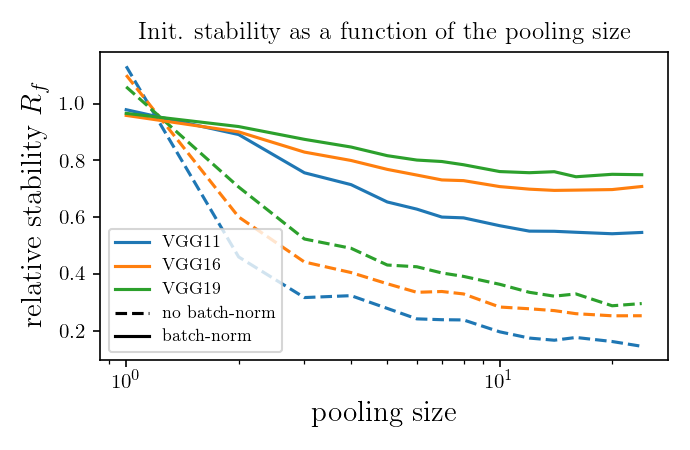
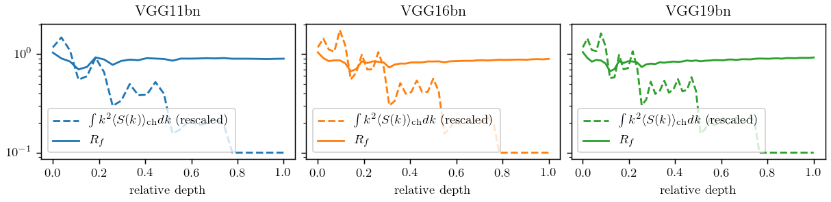
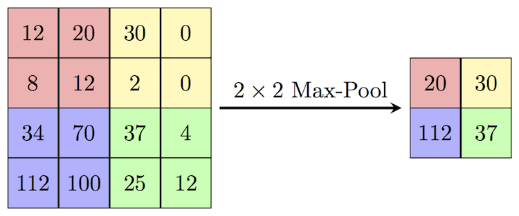
Filters actually learn to pool but other operations (e.g. ReLU) still make the spectrum more high freq.?
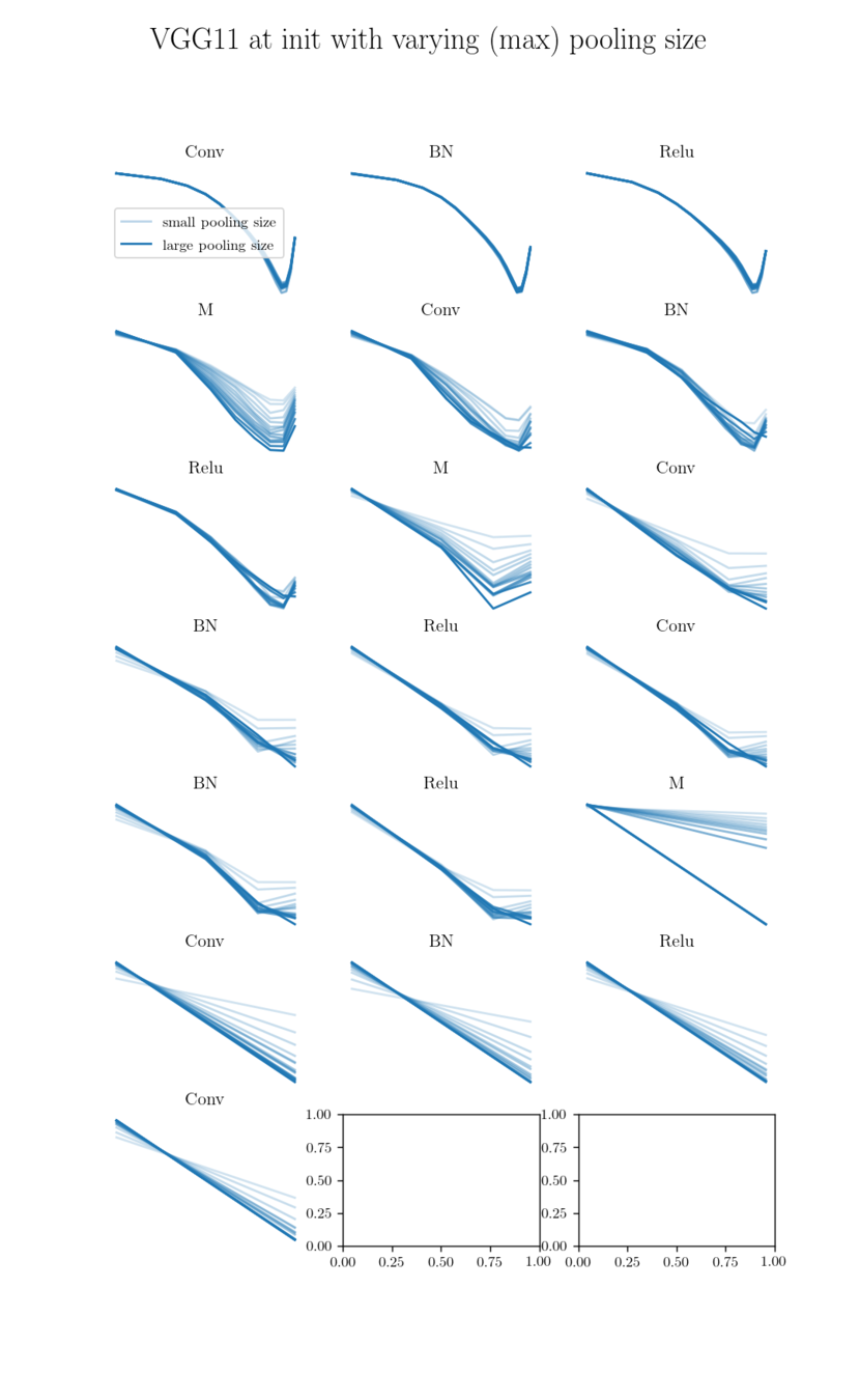
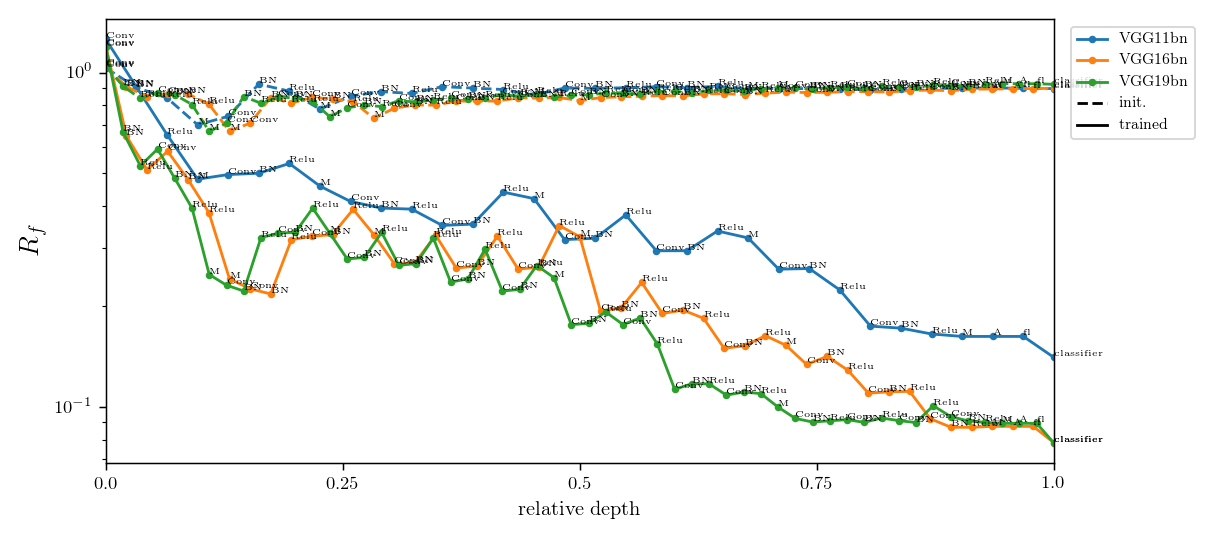
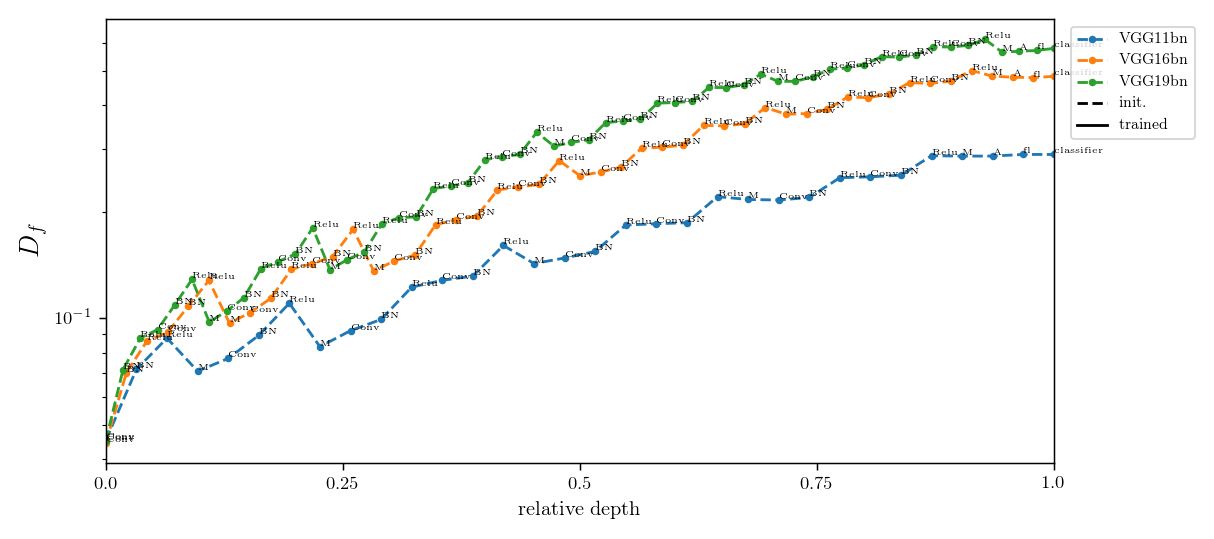
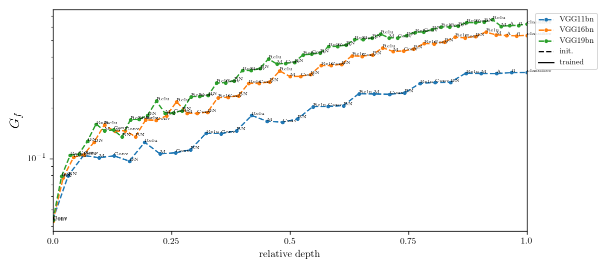
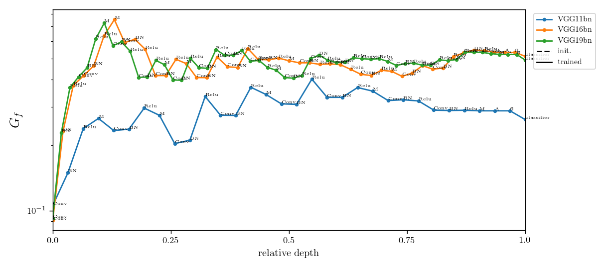
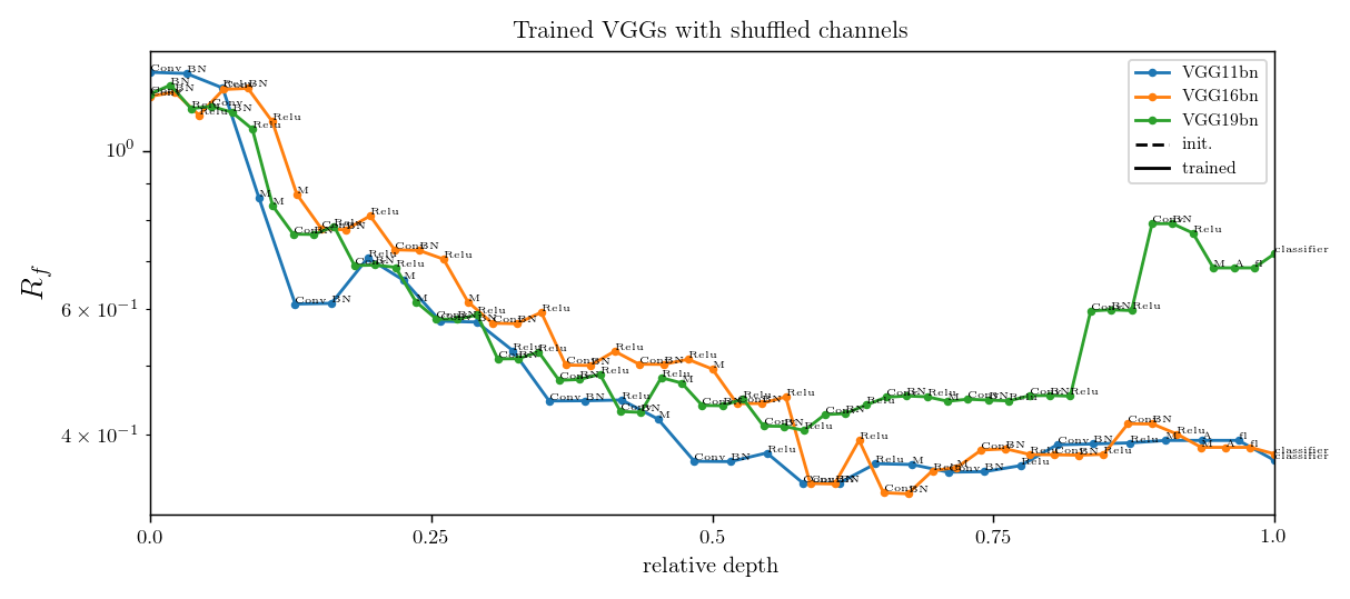
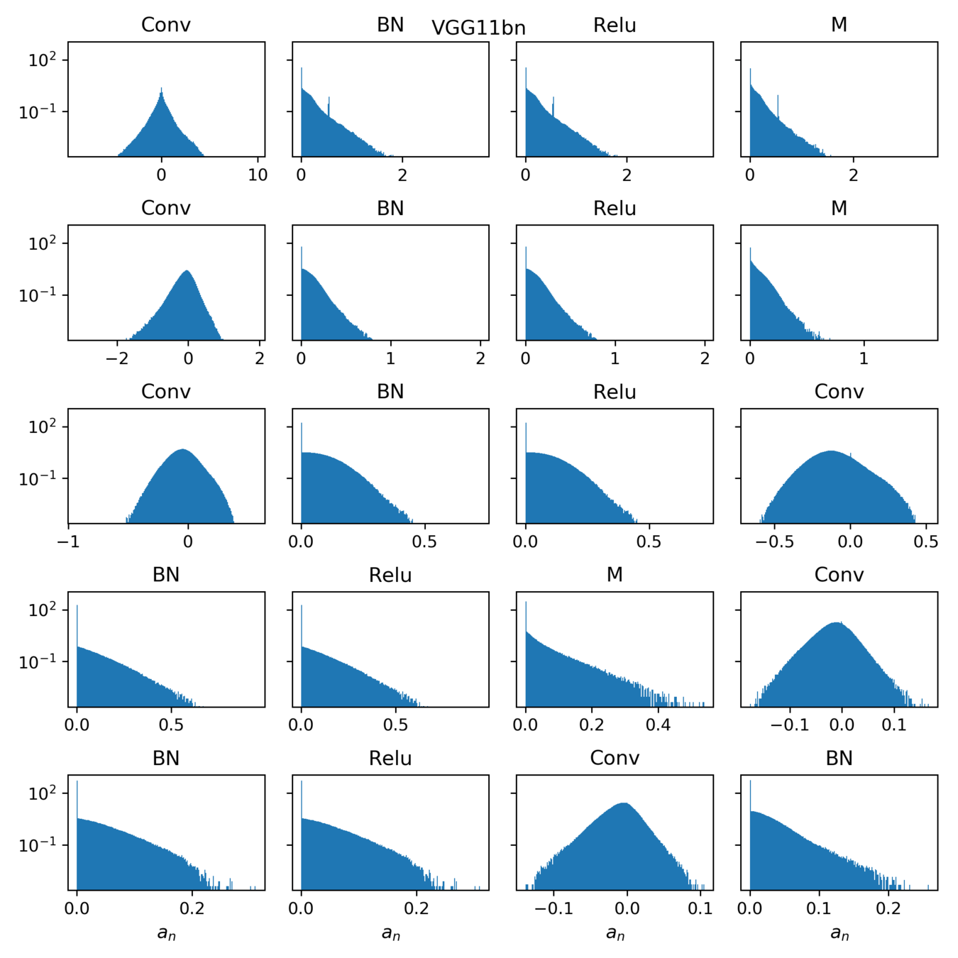
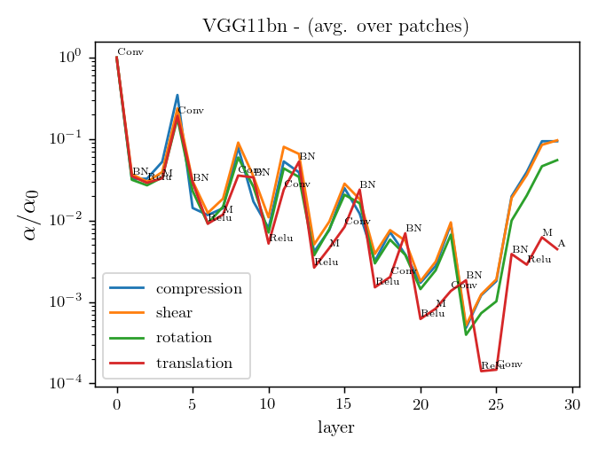
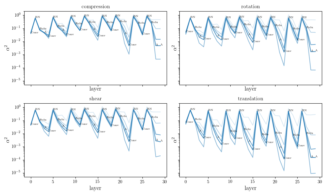
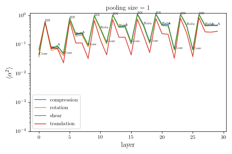
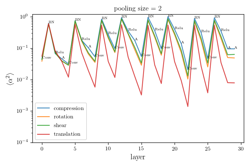
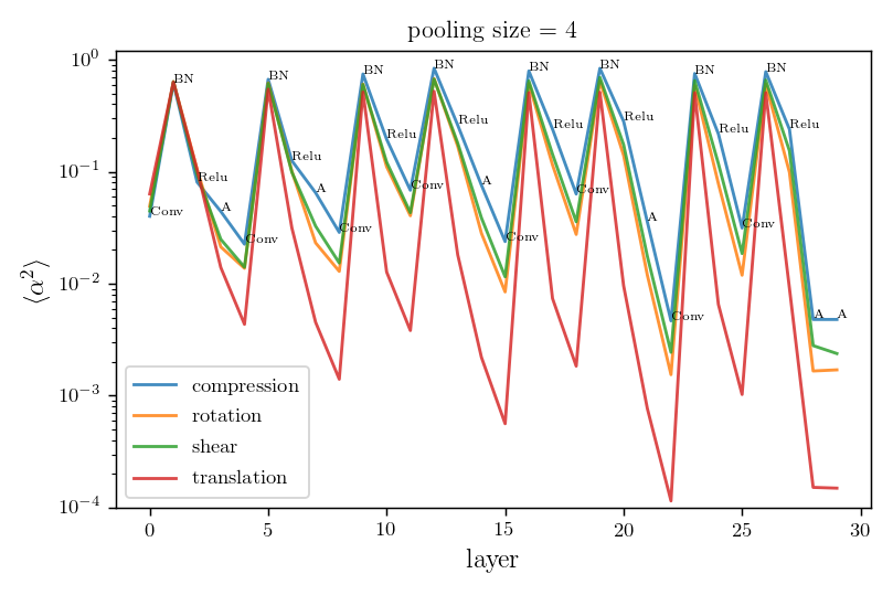
Relative stability after each operation (conv. batch-norm, ReLU, max-pool) inside VGGs
diffeo stability
init
trained
trained
init
noise stability
initialization:
trained:
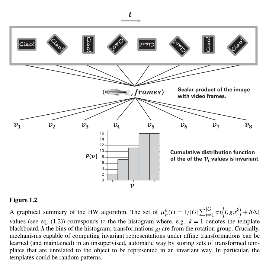
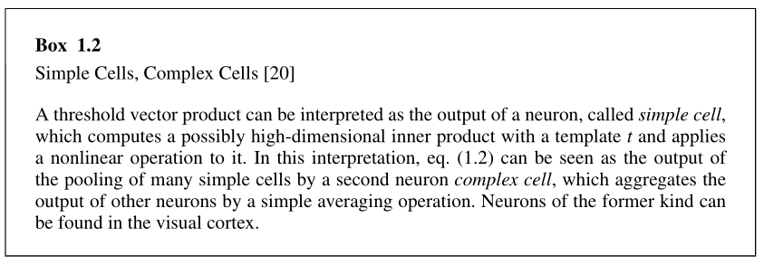
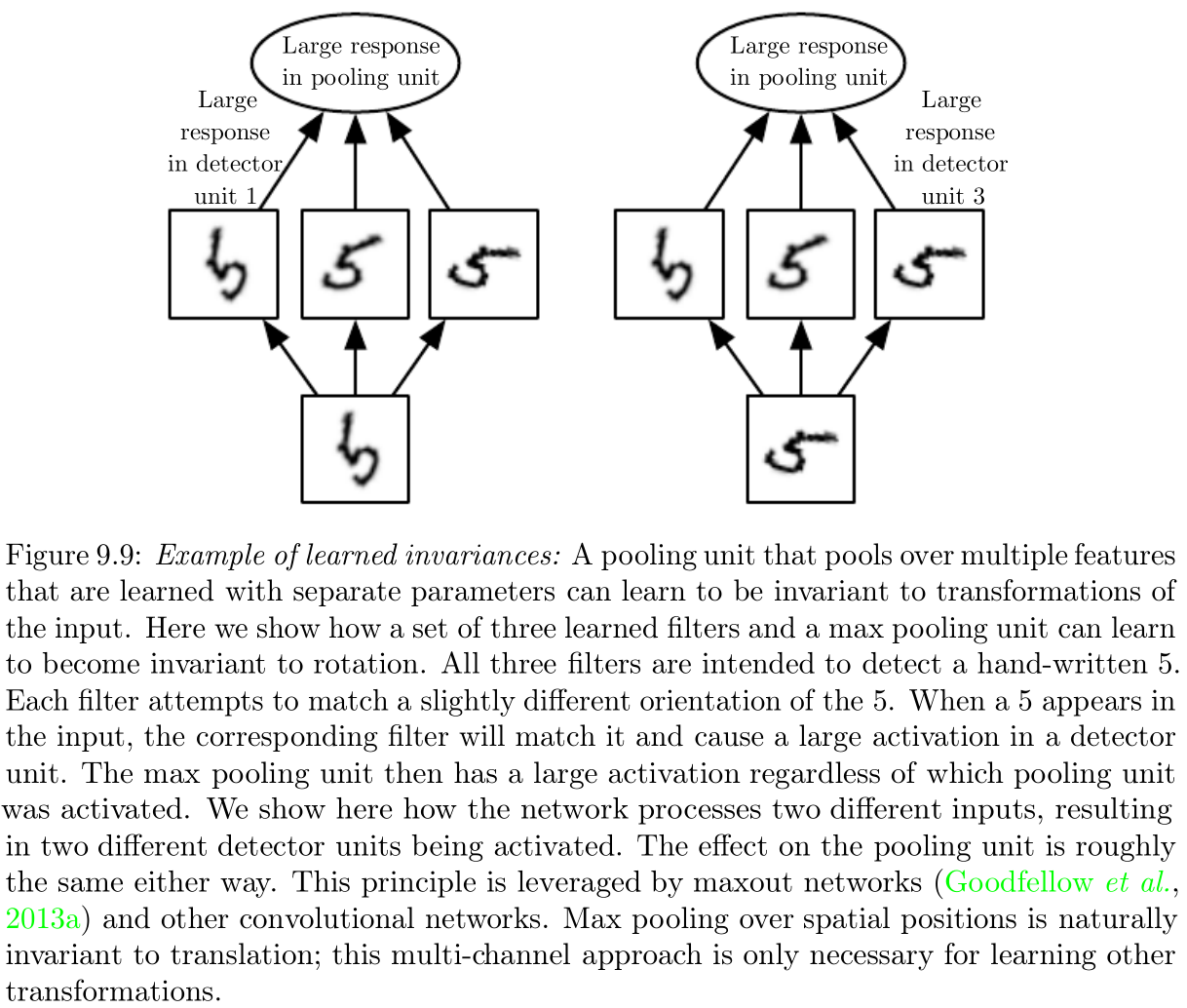
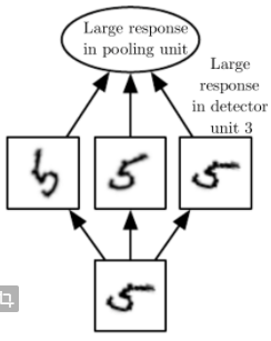
from Visual Cortex and Deep Networks by Poggio and Anselmi
Hypothesis 2:
Hyp. 1: Filters learn to pool
Hyp. 2: Say we want to implement rotational invariance with two layers of weights. One can do that by
This idea can also be found in neuroscience literature to explain how invariances are implemented in the visual cortex.
Can we test this idea by looking at subsequent layers of weights (say L1 and L2) and see if neurons in L2 are such that they couple neurons in L1 that do the same thing, up to a rotation?
from Visual Cortex and Deep Networks by Poggio and Anselmi
PCSL internal group meeting
November 11, 2021
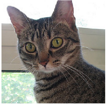
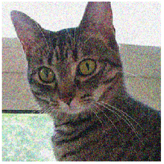
= "cat"
diffeo stability
additive noise stability
Hypothesis: nets become relatively stable by making filters low-pass with training.
We take a basis that is the eigenvectors of the Laplacian on the 3x3 grid and follow weigths evolution on each of the components and average over the channels:
$$c_{t, \lambda} = \langle (w_{\rm{ch}, t} \cdot \Psi_\lambda )^2\rangle_{\rm{ch}}$$
I plot $$\frac{c_{t, \lambda}}{c_{t=0, \lambda}}$$
We take a basis that is the eigenvectors of the Laplacian on the 3x3 grid and follow weigths evolution on each of the components and average over the channels:
$$c_{t, \lambda} = \langle (w_{\rm{ch}, t} \cdot \Psi_\lambda )^2\rangle_{\rm{ch}}$$
I plot $$\frac{c_{t, \lambda}}{c_{t=0, \lambda}}$$
Filters actually learn to pool!
What if we take a trained net and randomly permute the channels?
If it was all about (1), nothing should change.
Can we decouple the contribution of the two?
standard
shuffled channels
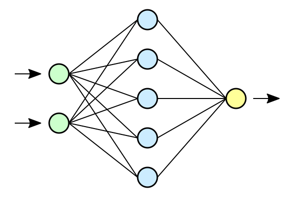
Take one hidden layer CNN or LCN, i.e.:
Can either train the whole net or just the FC layer.
Would this allow to say something about how the invariance is learned in these simple nets?
e.g. if only FC layer is trained, the net can only learn channel pooling and not spatial pooling.
Still, the net can still change spatial pooling by select the channels that are more low frequency...
only FC is trained
whole net is trained
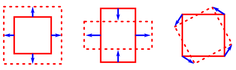
local translation
NOT a local translation
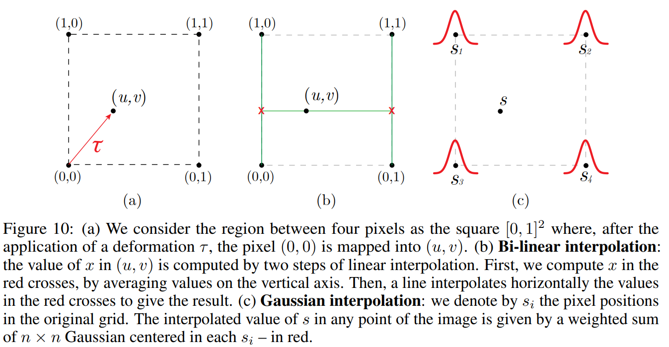
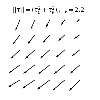
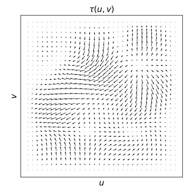
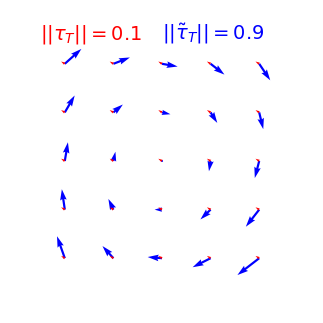
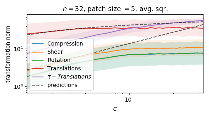
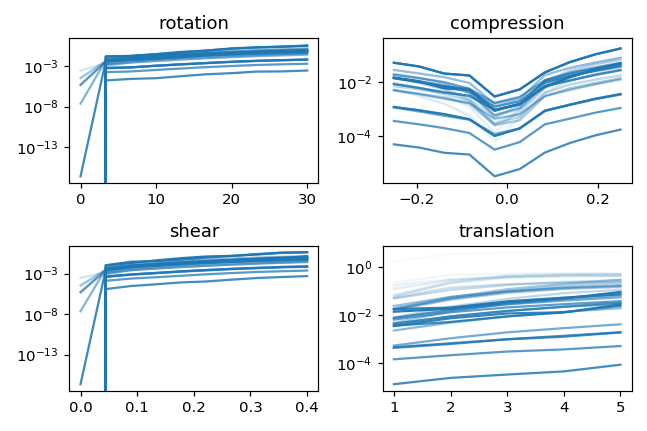
Which transformations make up the blue displacement field?
compression / expansion
pure shear
rotation
Locally, we can decompose our displacement field \(\tau(u, v)\) into translations, i.e. $$\langle\tau\rangle_\text{patch}$$
and linear transformations (i.e. defined by its 1st order derivatives):
Where
compression / expansion
pure shear
rotation
Example: compression / expansion
trace
symmetric traceless
antiymmetric
compression / expansion
pure shear
rotation
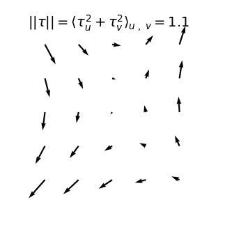
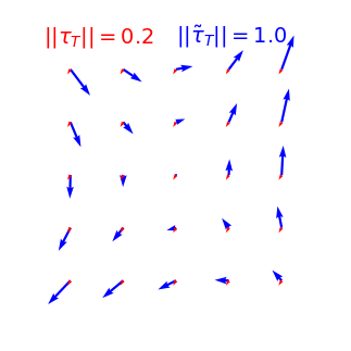
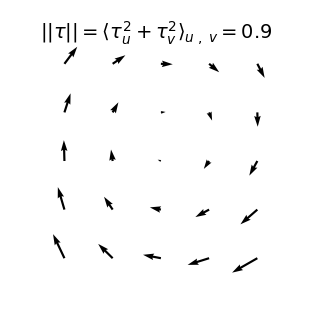
Our diffeo ensemble is defined as \(\tau = (\tau_u, \tau_v)\) with components
Where the norm of local translations can be computed as the average pixel displacement:
While the norm of each component of \(U\) reads
Compute the average of the norm (w/o the square)
Compute the empirical average over finite patches
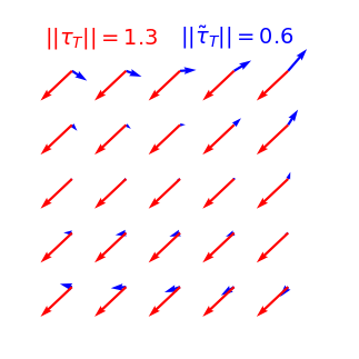
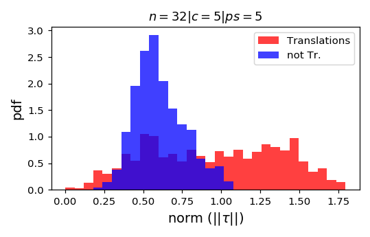
We can compute the norm of the part of \(\tau\) that is not a translation (on a patch):
As we take a finite patch size, it's not ok anymore!
https://journals.aps.org/pre/pdf/10.1103/PhysRevE.95.032401
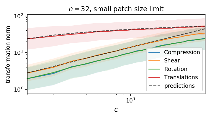
Is diffeo relative stability achieved also by getting locally invariant to the other linear transformations
(i.e. rotation, compression, pure shear)?
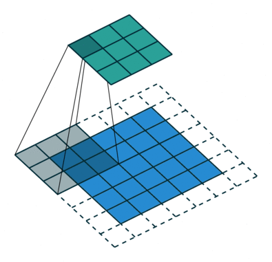
convolution layer
VGG11
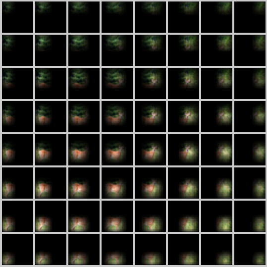
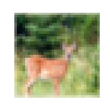
8x8 activation map receptive field
input
8x8x256
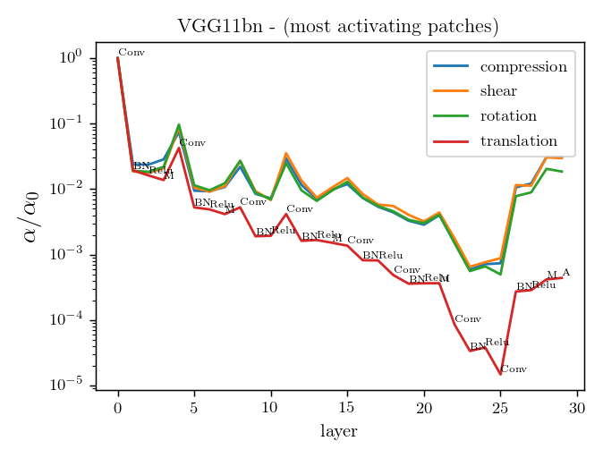
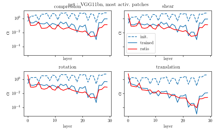
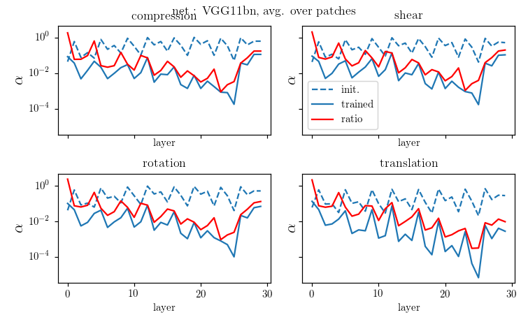
We can measure neurons' stability to linear transformations by deforming locally what's in the their receptive field!!
We compare local translations, rotations, compressions, pure shears, by fixing their norm to 1, i.e. $$\delta = \|R\| =\|C\| =\|S\| = 1.$$
We compute the average neurons stability as
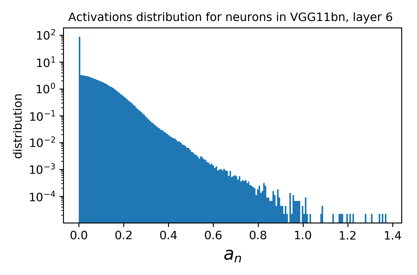
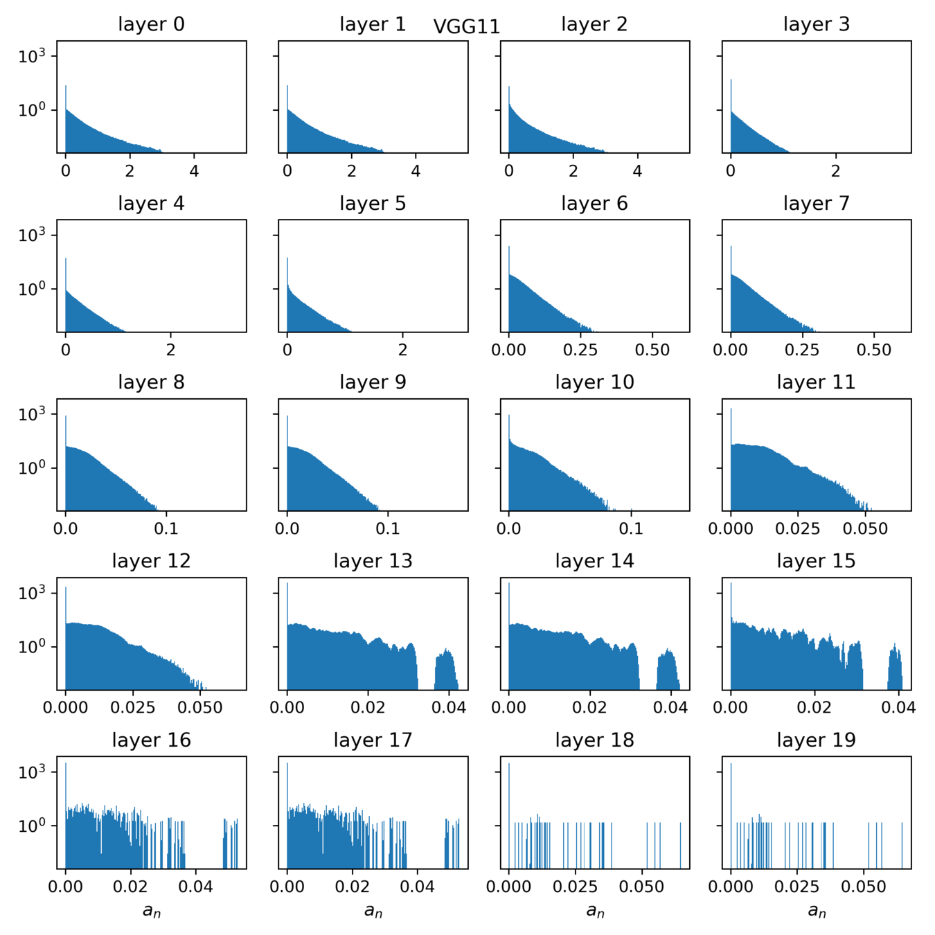
where \(a_n\) is the activation of neuron \(n\) on patch \(x\). The neurons' stability \(\alpha\) can be measured for each layer.
Note:
Is it a fair comparison..?
Side note: each deformation, being applied locally to a single receptive field, depends on the neuron we are measuring. As a consequence, to measure \(\alpha\), one needs to do one forward pass per image per neuron, and to get some statistics over inputs gets very expensive.
This could be an issue if neurons are only active on a few patches, i.e. when they detect something.
Solutions..?
issues:
a few random patches
max response patch
Average over the top n response patches?
rotation
translation
receptive field
object
r.f. center
For neurons deep in the net, receptive fields are large and the effect of different transformations can start to mix up.
Pixels displacement field along \(x\):
where Fourier coefficients are sampled from
PCSL retreat
December 2021
By Leonardo Petrini


