


Leonardo Petrini
PhD Student @ Physics of Complex Systems Lab, EPFL Lausanne
Candidate: Leonardo Petrini
Exam jury:
Prof Hugo Dil, président du jury
Prof Matthieu Wyart, directeur de thèse
Prof Florent Krzakala, rapporteur
Prof Andrew Saxe, rapporteur
Prof Nathan Srebro, rapporteur
September 12, 2023
(supervised learning)
correct prediction?
?
model + algorithm
model + algorithm
tune the model to make correct predictions on training data
0 1
0 1
0 1
Example for \(\epsilon = 1/3\):
\(P = 3 \text{ in } d = 1\)
\(P = 9 \text{ in } d = 2\)
\(P = 27 \text{ in } d = 3 \dots\)
Language, e.g. ChatGPT
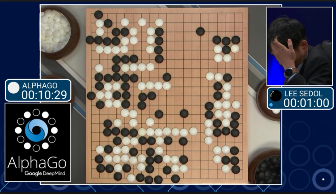
Go-playing
Autonomous cars
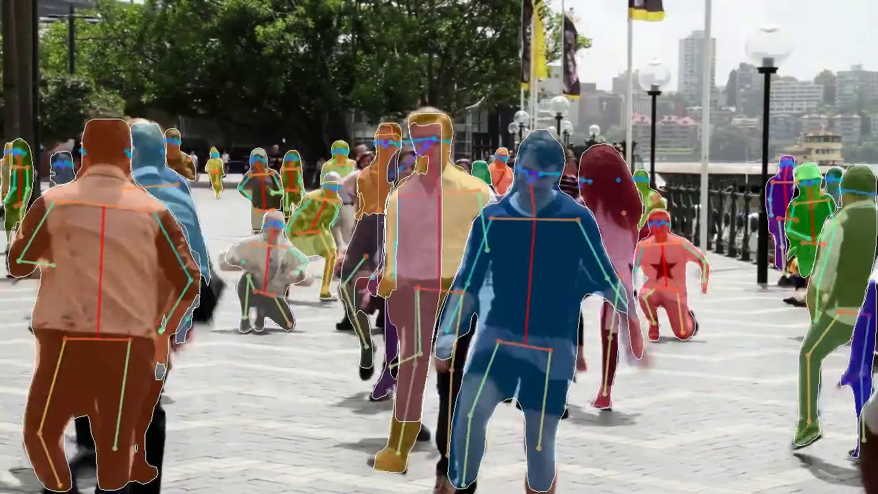
Pose estimation
etc...
data manifold
Pope et al. '21
Goodfellow et al. (2009); Bengio et al. (2013); Bruna and Mallat (2013); Mallat (2016)
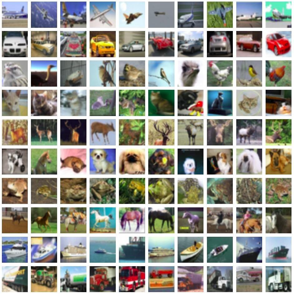
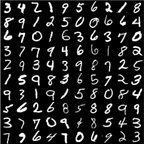
Deng et al. '09
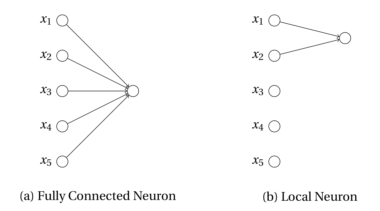
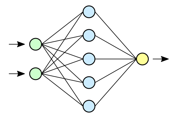
Shallow fully-connected networks (FCNs) with ReLU activations,$$f(\bm{x}) = \frac{1}{H} \sum_{h=1}^H w_h \sigma( \bm{\theta}_h\cdot\bm{x}) $$
$$H: \text{width}$$
$$d: \text{input dimension}$$
$${\bm \theta}: \text{1st layer weights}$$
$$\omega: \text{2nd layer weights}$$
$$\sigma: \text{activation function}$$
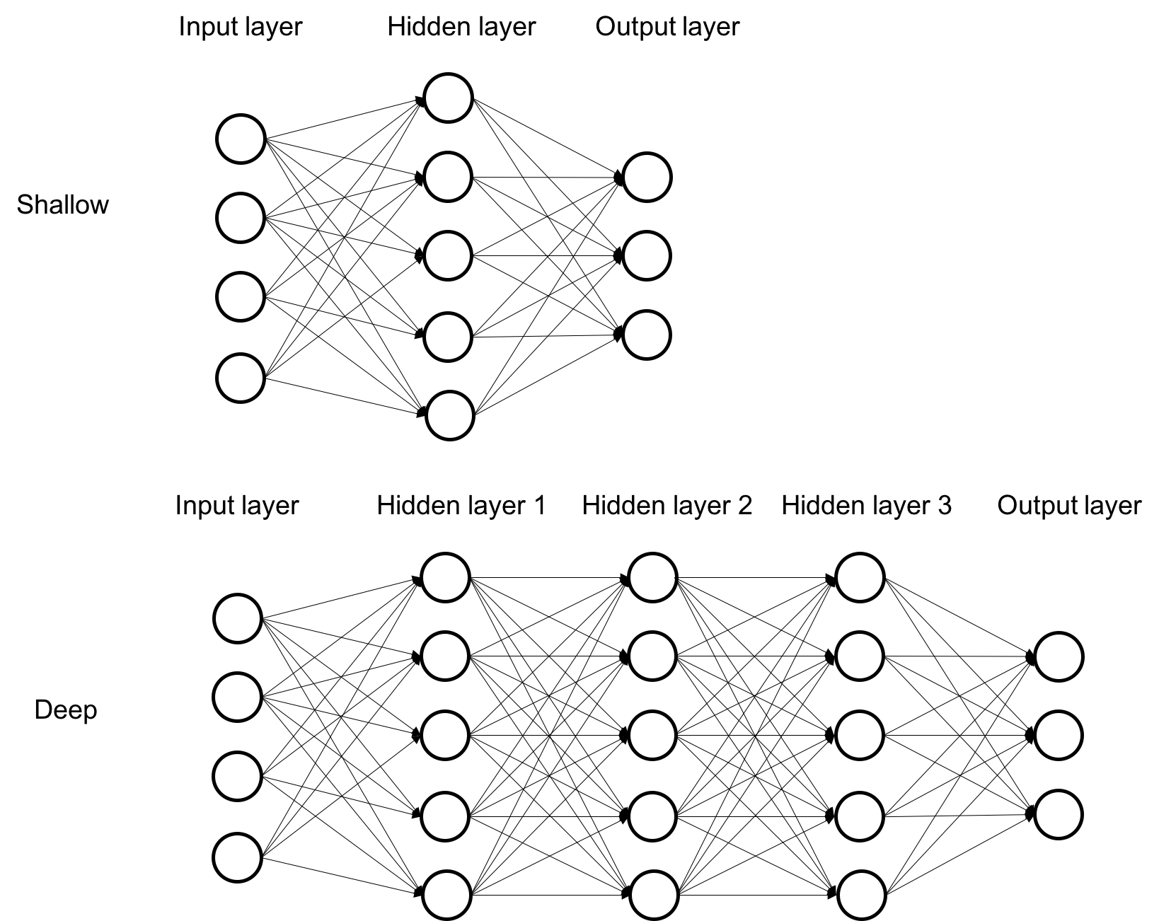
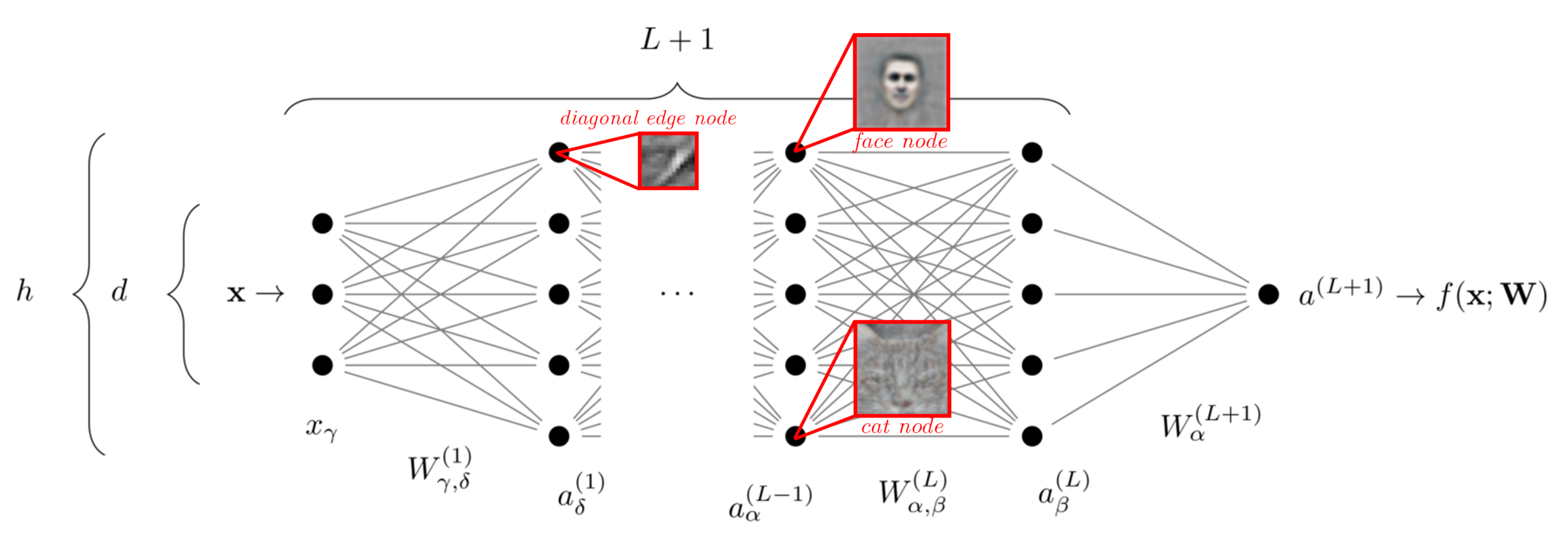
network depth
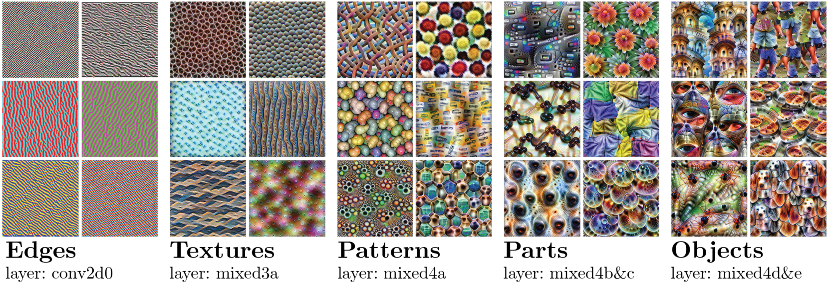
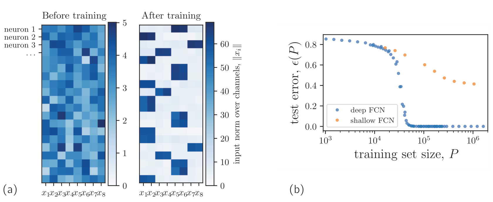
Figure: inputs that maximally activate neurons at a given layer:
Zeiler and Fergus (2014); Yosinski et al. (2015);
Olah et al. (2017)
Ansuini et al. '19; Recenatesi et al. '19
Ansuini et al. '19
Recenatesi et al. '19
adapted from Lee et al. '13
How dimensionality reduction affects performance?
Lazy Regime
Feature Regime
Jacot et al. (2018); Chizat et al. (2019); Bach (2017); Mei et al. (2018); Rotskoff and Vanden-Eijnden (2018); [...]
The same neural network architecture can be trained in two regimes, depending on initialization scale. Regimes are well characterized at infinite width.
(also NTK regime)
(also rich / hydrodynamic / mean-field / active)
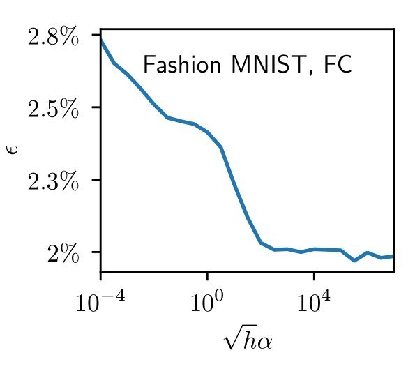
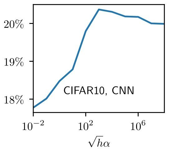
How does operating in the feature or lazy regime affect neural nets performance?
Each regime can be favoured by different architectures and data structures [Geiger et al. 2020b]:
Test error
feature lazy
Test error
feature lazy
MNIST, CNN
\(\epsilon\)
Chizat and Bach (2018);
Geiger et al. (2020b, 2021);
Novak et al. (2019);
Woodworth et al. (2020)...
algo: gradient descent
init. scale,
often power law in practice
Hestness et al. (2017); Spigler et al. (2020); Kaplan et al. (2020)
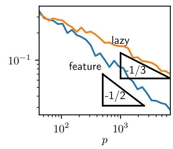
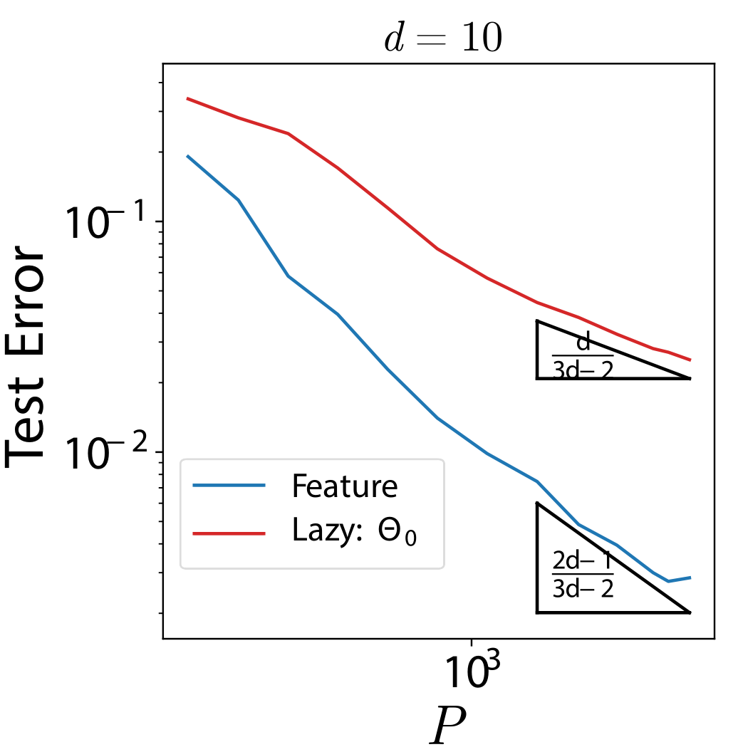
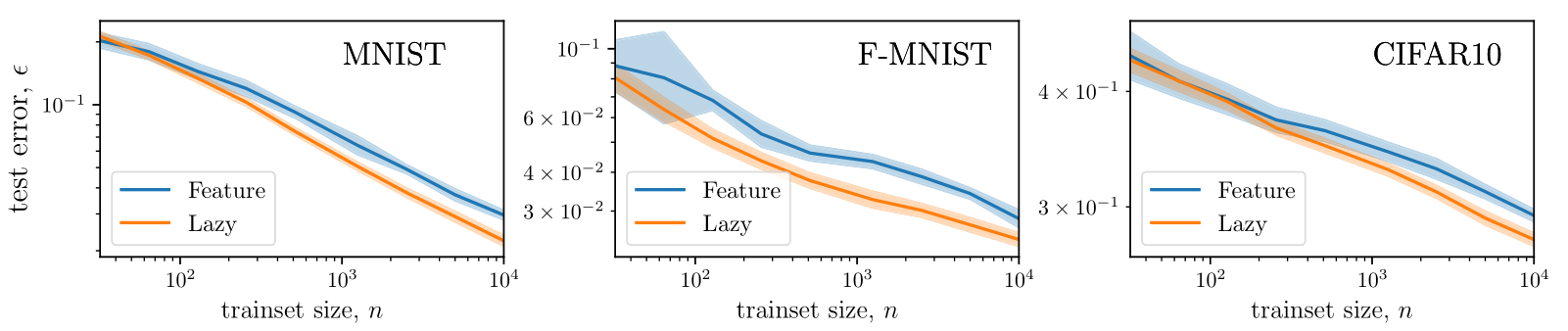
Moreover, if we look at gen. error vs. num. training points:
we measure a different exponent \(\beta\) for the two regimes.
In the following, we will often use \(\beta\) to characterize performance.
test error
train. set size
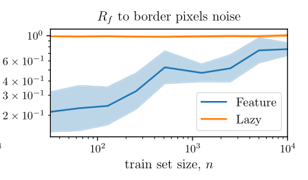
We study interplay between data invariances
and neural networks architectures:
irrelevant pixels
Barron (1993); Bach (2017); Chizat and Bach (2020); Schmidt-Hieber (2020); Yehudai and Shamir (2019); Ghorbani et al. (2019, 2020); Wei et al. (2019)...
The target function is highly anisotropic, in the sense that it depends only on a linear subspace of the input space:
$$ f^*(\bm x) = g(A{\bm x}) \quad\text{where}\quad A\,\, : \mathbb{R}^d \to \mathbb{R}^{d'} \quad \text{and} \quad d' \ll d. $$
Barron (1993); Bach (2017); Chizat and Bach (2020); Schmidt-Hieber (2020); Yehudai and Shamir (2019); Ghorbani et al. (2019, 2020); Wei et al. (2019)...
Animation: weights evolution during training
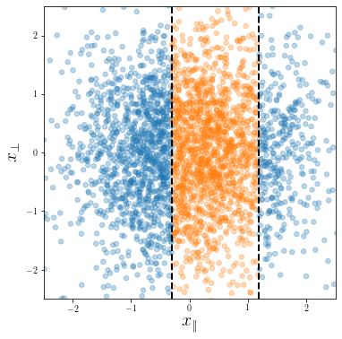
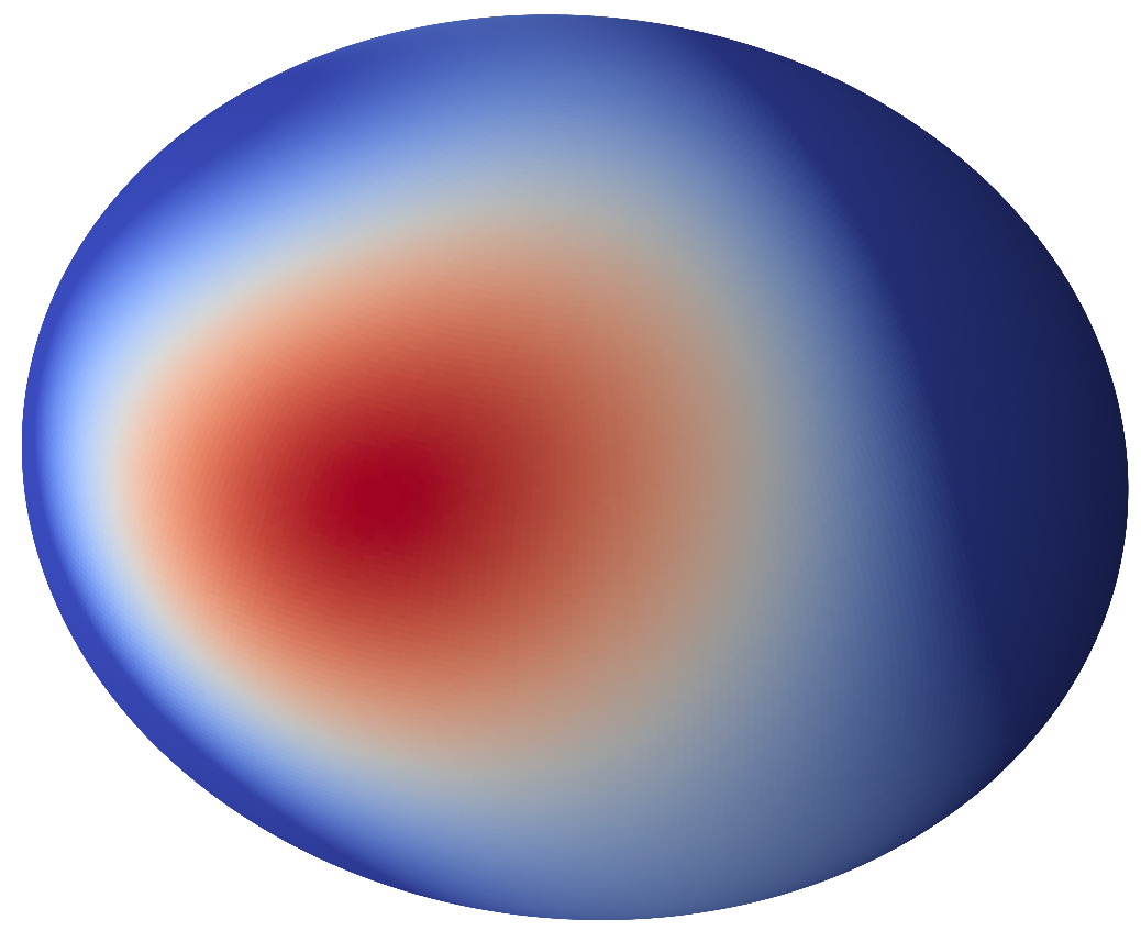
Simple model of data for a task (approximately) invariant to rotations,
e.g. \({\bm x}\) uniform on the circle and regression of \(f^*({\bm x}) = 1\):
Example: \(d=3\), large \(\nu_t\)
LP, Cagnetta et al. 2022
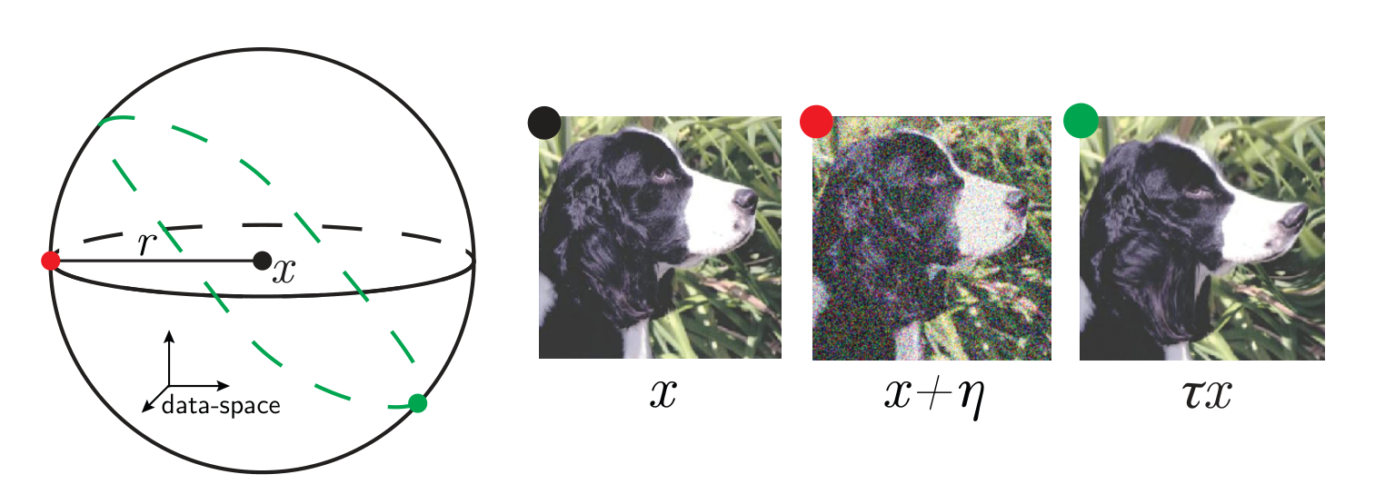
Bruna and Mallat '13, Mallat '16
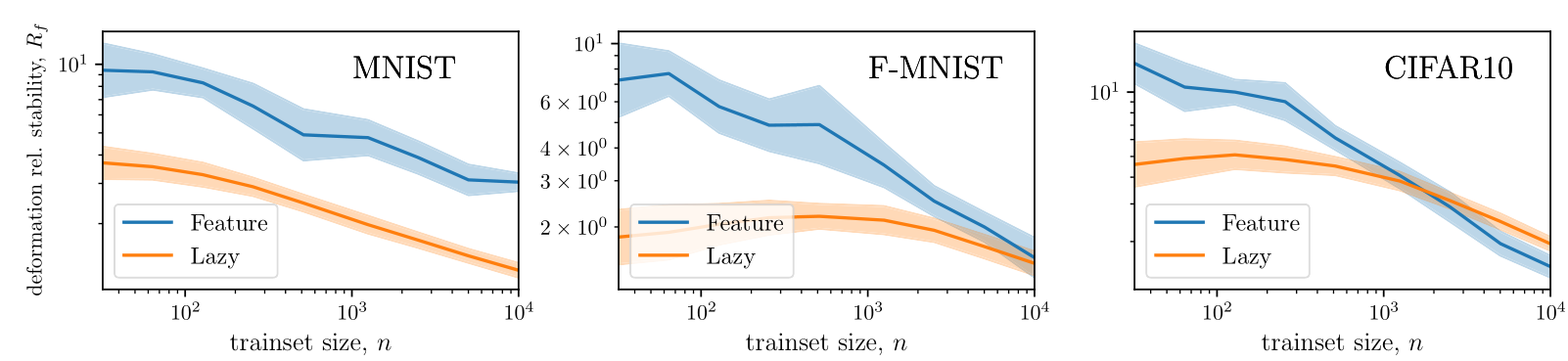
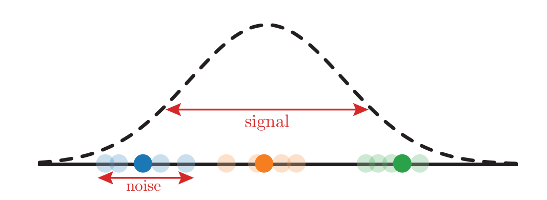
Invariance measure: relative stability
(normalized such that is =1 if no diffeo stability)
we introduced a model to generate deformations of controlled magnitude
Geiger et al. (2020a,b); Lee et al. (2020)
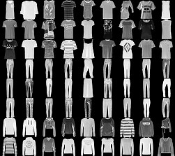
Figure. Lazy predictor is smoother along diffeomorphisms for image classification.
more smooth
Fashion MNIST
more invariant
initialization: \(R_f \sim 1\)
Mossel '16; Poggio et al. '17; Malach and Shalev-Shwartz '18, '20; LP et al '23;
Bruna and Mallat '13, LP et al. '21, Tomasini, LP et al. '22;
...
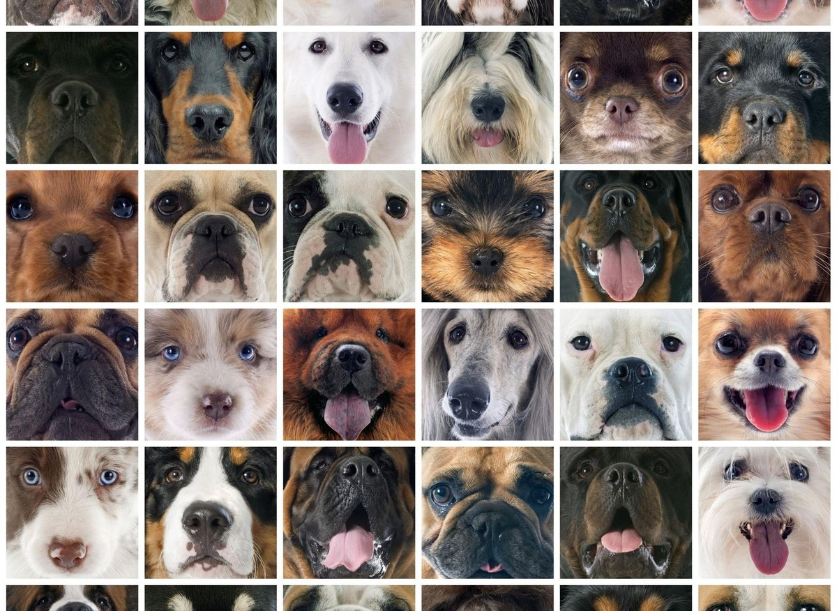
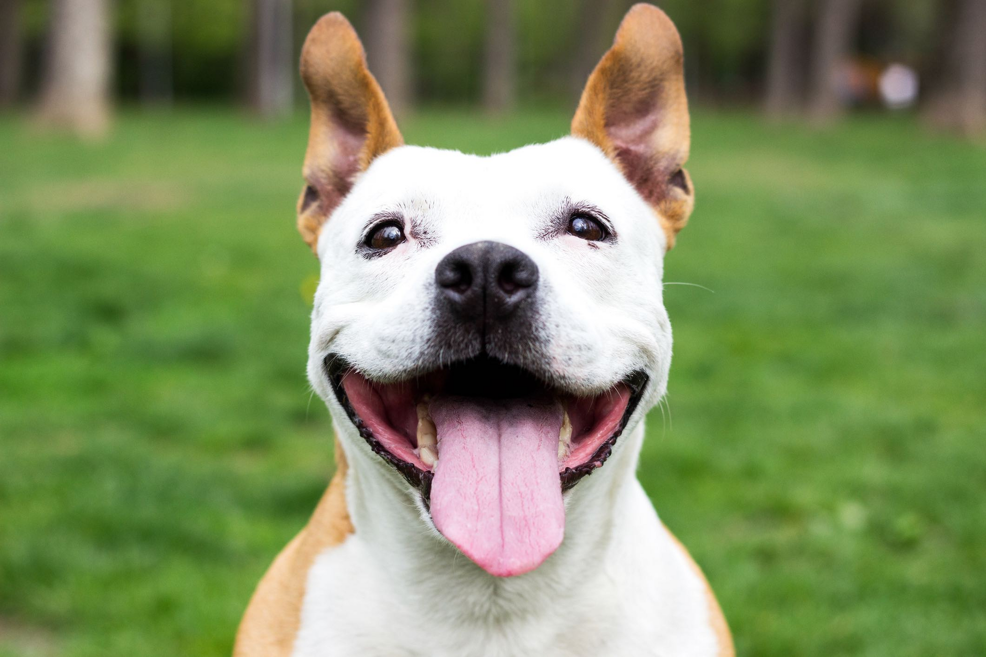
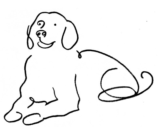
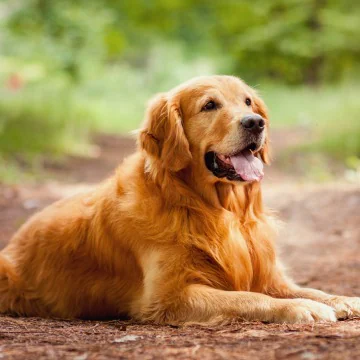
dog
face
paws
eyes
nose
mouth
ear
edges
text:
images:
irrelevant pixel
Barron '93; Bach '17; Chizat and Bach '20; Schmidt-Hieber '20; Ghorbani et al. '19, '20; Paccolat, LP et al. '20; [...]
...
dog
face
paws
eyes
nose
mouth
ear
edges
Previous works:
Poggio et al. '17
Mossel '16, Malach and Shalev-Shwartz '18, '20
Open questions:
Physicist approach:
Introduce a simplified model of data
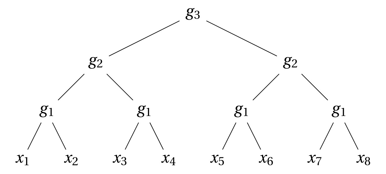
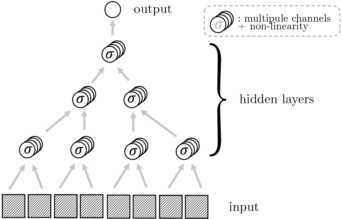
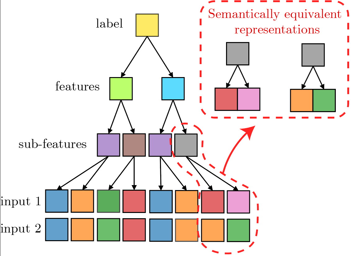
We consider hierarchically compositional and local tasks of the form: $$f^*({\bm x}) = g_3(g_{2}(g_{1}(x_1, x_2), g_{1}(x_3, x_4)), g_{2}(g_{1}(x_5, x_6), g_{1}(x_7, x_8))).$$
Depth
\(L=3\)
locality: \(s=2\)
input size: \(d = s^L\)
Example: \(m=v=s=2\)
Starting from outputs:
can use it as generative model
How to choose the \(g_l\)'s?
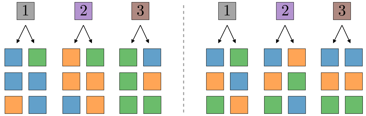
\(g_l\) for \(m=2, v=3, s=2\)
The constituent functions \(g_l\) are chosen uniformly at random:
randomly assign \(m\) input patches in \(V^s\) to each of the \(v\) outputs.
synonyms
Can generate samples starting from outputs!
Simple example with \(m=v=2\)
Patches of dim. \(s=2\)
The constituent functions \(g_l\) are chosen uniformly at random:
randomly assign \(m\) input patches in \(V^s\) to each of the \(v\) outputs.
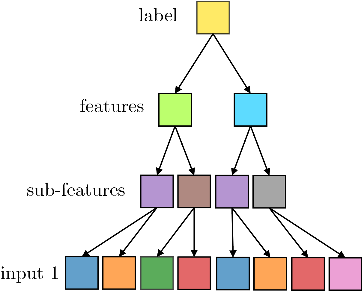
label 2
lower level features
inputs
intermediate
representations
start from labels:
label 1
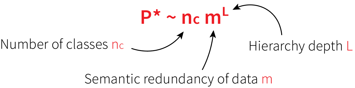
How many points do neural networks need to learn these tasks?
in practice: one-hot encoding of input features/color
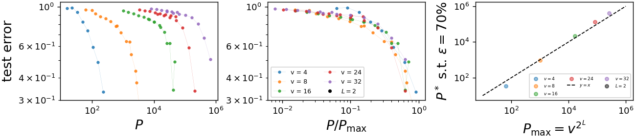
Training a shallow fully-connected neural network
with gradient descent to fit a training set of size \(P\).
original
rescaled \(x-\)axis
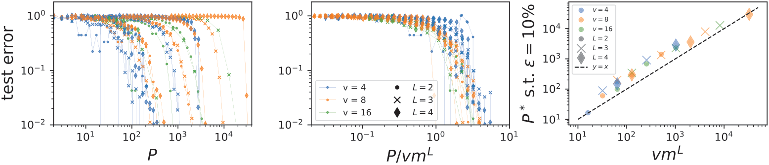
Training a deep convolutional neural networks with \(L\)
hidden layers on a training set of size \(P\).
original
rescaled \(x-\)axis
Can we understand DNNs success?
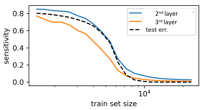
Are they learning the structure of the data?
How is synonymic invariance learned?
= sample complexity of DNNs!!
Main takeaway: neural networks can profitably learn data invariances in the feature regime, provided the right architecture.
Some open questions:
Neyshabur (2020); Pellegrini and Biroli (2021); Ingrosso and Goldt (2022)
RHM
Sparse RHM
Tomasini at al. (in preparation)
By Leonardo Petrini


