

Leonardo Petrini
PhD Student @ Physics of Complex Systems Lab, EPFL Lausanne
Leonardo Petrini @ PCSL Group Meeting - July 16th, 2020.
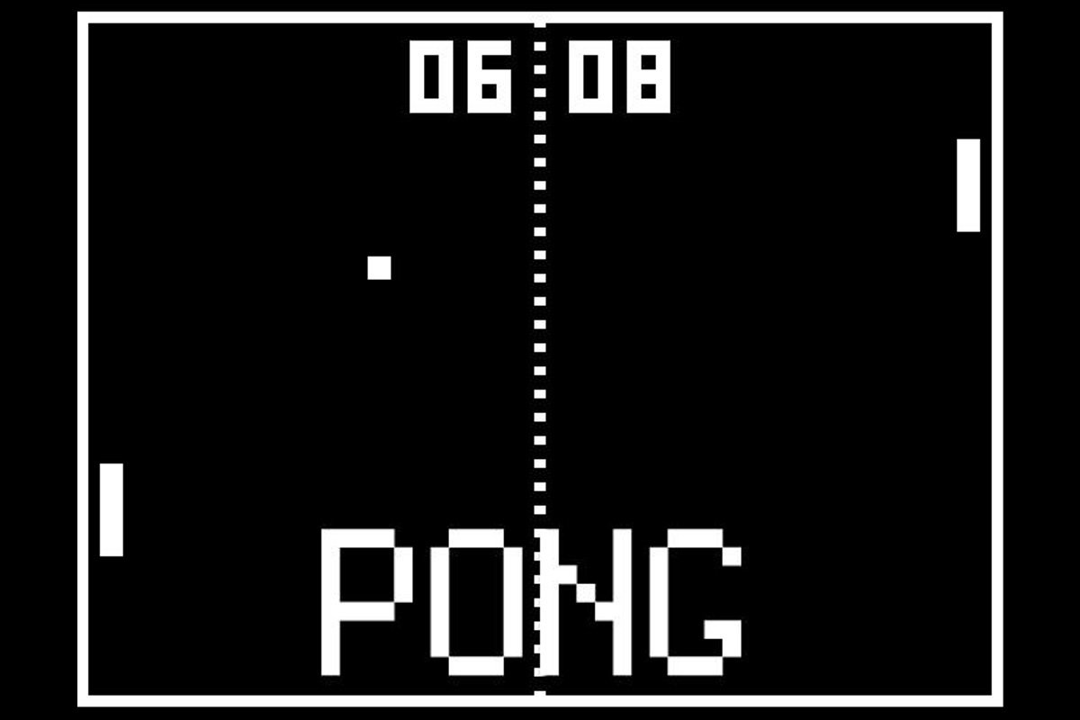
Motivation: the game of Pong
How to make a computer play pong?
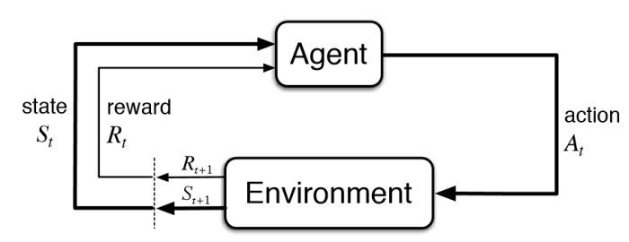
RL ingredients
e.g. (Game of Pong)
(there is some Markovian assumption here)
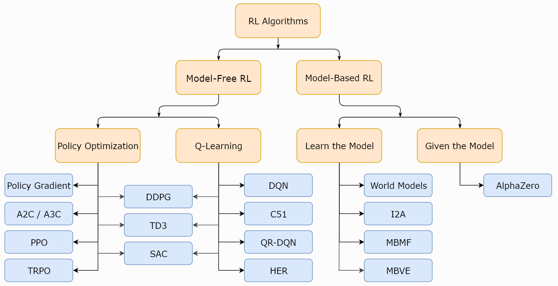
A Taxonomy of RL Algorithms
spinningup.openai.com
2
3
1
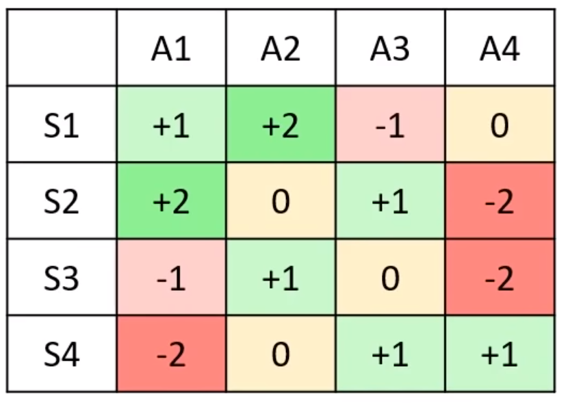
Agent's cheat sheet:
For each state \(s_t\), take action \(a_t = \argmax_a \text{TABLE}(s_t, a)\)
Q-values and Policy (1)
Agent's cheat sheet:
For each state \(s_t\), take action \(a_t = \argmax_i \text{TABLE}(s_t, a_i)\)
Q-values and Policy (1)
}
}
Policy
Q-values
Q-values and Policy (2)
Q-value: expected discounted reward for playing action \(a\) in state \(s\)
$$\begin{aligned}Q(s_t,a_t) &\stackrel{.}{=} \langle r_t + \gamma r_{t+1} + \gamma^2 r_{t+2}+ \dots \rangle, \\ &\end{aligned}$$
\(\gamma < 1\) is the discount factor.
Policy: probability of playing action \(a\) in state \(s\) $$\pi(a|s)$$
Q-values and Policy (2)
Q-value: expected discounted reward for playing action \(a\) in state \(s\)
$$\begin{aligned}Q(s_t,a_t) &\stackrel{.}{=} \langle r_t + \gamma r_{t+1} + \gamma^2 r_{t+2}+ \dots \rangle\: \\ &= \langle r_t \rangle + \gamma Q(s_{t+1}, a_{t+1}),\end{aligned}$$
\(\gamma < 1\) is the discount factor.
Policy: probability of playing action \(a\) in state \(s\) $$\pi(a|s)$$
algo to exploit
this equality
SARSA and Q-learning
$$s \rightarrow a \rightarrow r \rightarrow s' \rightarrow a' $$
SARSA algorithm. Initialize Q-values and start from state \(s_0\)
(1) choose action \(a\) according to policy \(\pi(a|s)\) \(-\) e.g. greedy: choose \(a^* = \argmax_a Q(s,a)\)
(2) observe \(r\) and \(s'\)
(3) choose action \(a'\) according to \(\pi(a'|s')\)
(4) update with SARSA rule:
$$\Delta Q(s,a) = \eta [r + \gamma Q(s',a') - Q(s,a)]$$
(5) \(s \leftarrow s', a \leftarrow a'\)
(6) go to (1)
Q-learning
Q-learning algorithm (off-policy)
Initialize Q-values and start from state \(s_0\)
(1) choose action \(a\) according to policy \(\pi(a|s)\) \(-\) e.g. greedy: choose \(a^* = \argmax_a Q(s,a)\)
(2) observe \(r\) and \(s'\)
(3) update with Q-learning rule:
$$\Delta Q(s,a) = \eta [r + \gamma \max_{a'} Q(s',a') - Q(s,a)]$$
(5) \(s \leftarrow s', a \leftarrow a'\)
(6) go to (1)
Discrete vs continuous state space
What if the state space is too large, or even continuous?
We could use a neural network to approximate the Q-value function!!
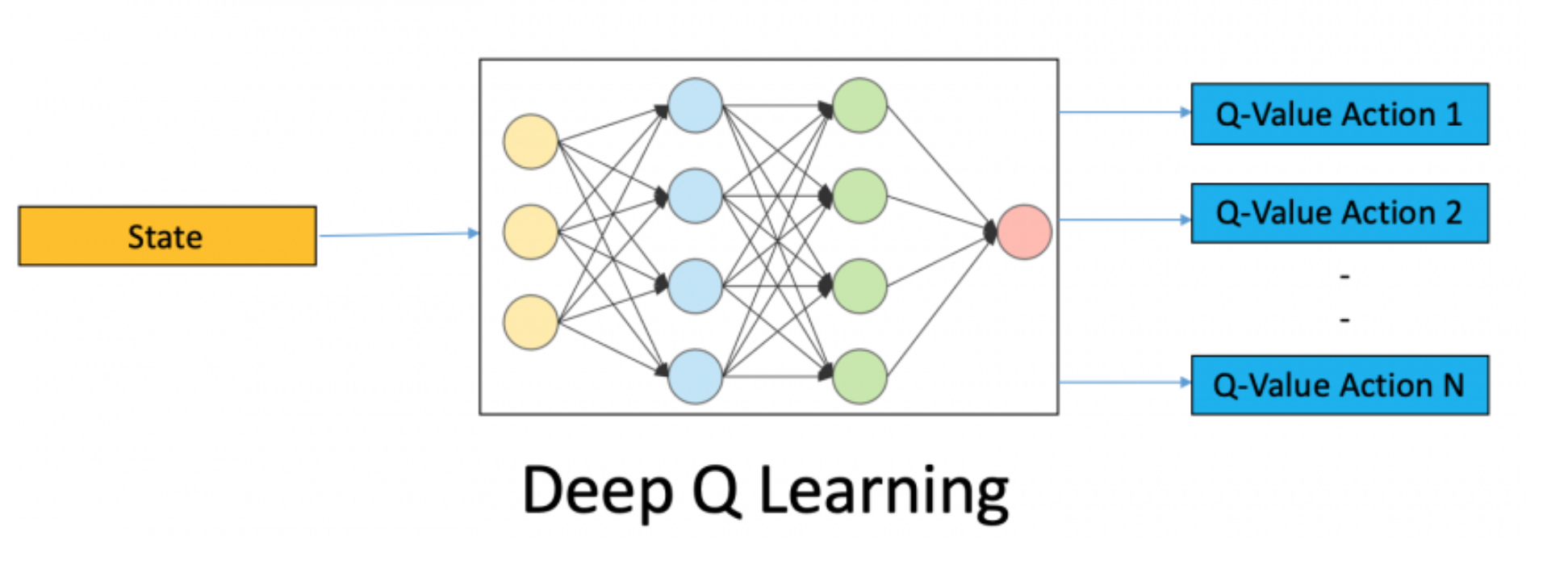
Deep Q-learning (DQN)
Use a neural network to learn Q-values.
Output vector \(\{Q\)\(_w\)\((a_n,s)\}_{n=1}^N\), where \(w\) are the network parameters.
Loss function (from SARSA update rule):
$$\mathcal{L} = \frac{1}{2} [r + \gamma Q_w(s',a') - Q_w(s,a)]^2$$
Deep Q-learning (DQN)
Use a neural network to learn Q-values.
Output vector \(\{Q\)\(_w\)\((a_n,s)\}_{n=1}^N\), where \(w\) are the network parameters.
Loss function (from SARSA update rule):
$$\mathcal{L} = \frac{1}{2} [r + \gamma Q_w(s',a') - Q_w(s,a)]^2$$
The target changes during learning, extra care needed!!
}
Target. Ignore \(w\) dependence
x
Yes, we can!
Policy Gradient
Goal: approximate the optimal policy function \(\pi^*(a|s)\)
We do that by parametrizing the policy \(\pi_\theta(a|s)\) and optimize \(\theta\) in order to maximize a performance measure \(J(\theta)\).
\(\rightarrow\) Gradient Ascent in parameter space:
$$\theta_{n+1} = \theta_n + \eta \nabla_\theta J(\theta)$$
Policy Gradient (2)
What performance measure?
Total expected reward for playing an episode of the game following a trajectory \(\tau = \{s_0, \dots s_{end}\}\),
$$J(\theta) = \mathbb{E}_{\tau | \pi_\theta}[r(\tau)]$$
We define $$\pi_\theta(\tau) \stackrel{.}{=} p(s_0)\,\Pi_{t=0}^T p(s_{t+1}| s_t, a_t)\pi_\theta(a_t|s_t)$$
How do we deal with the gradient of an expectation?
Policy Gradient
Goal: approximate the optimal policy function \(\pi^*(a|s)\)
We do that by parametrizing the policy \(\pi_\theta(a|s)\) and optimize \(\theta\) in order to maximize a performance measure \(J(\theta)\).
\(\rightarrow\) Gradient Ascent in parameter space:
$$\theta_{n+1} = \theta_n + \eta \nabla_\theta J(\theta)$$
Performance measure? Total expected reward for playing an episode of the game following a trajectory \(\tau = \{s_0, \dots s_{end}\}\),
$$J(\theta) = \mathbb{E}_{\tau | \pi_\theta}[r(\tau)]$$
We define $$\pi_\theta(\tau) \stackrel{.}{=} p(s_0)\,\Pi_{t=0}^T p(s_{t+1}| s_t, a_t)\pi_\theta(a_t|s_t)$$
How do we deal with the gradient of an expectation?
Policy Gradient Theorem (1)
$$ $$
The derivative of the expected reward is the expectation of the reward times the derivative of the log policy:
Policy Gradient Theorem (2)
$$ $$
Recall: \(\pi\)\(_\theta\)\((\tau) \stackrel{.}{=} p(s_0)\,\Pi_{t=0}^T p(s_{t+1}| s_t, a_t)\)\(\pi_\theta(a_t|s_t)\)
The gradient of the performance function finally reads
No need to know about the initial state distribution or the transition probabilities between states!!
REINFORCE algorithm
$$ $$
Performance measure gradient:
Trajectory reward \(r(\tau)\) ?
The REINFORCE algorithm takes the discounted return
$$r(\tau) = \sum_{t=0}^T G_t = \sum_{t=0}^T (r_t + \gamma r_{t+1} + \gamma^2 r_{t+2} + \dots )$$
Interpretating \(\Delta\theta \varpropto G_t \frac{\nabla_\theta\pi_\theta (a_t|s_t)}{\pi_\theta(a_t|s_t)}\) : if taking action \(a_t\) in state \(s_t\) gives positive return \(\rightarrow\) move \(\theta\) in the direction that increases the probability of repeating \(a_t\) when visiting \(s_t\).
Issue. Rewards are usually sparse \(\rightarrow\) average over trajectories have high variance.
REINFORCE w/ baseline
To lower the variance we can add a baseline
$$\Delta\theta \varpropto (G_t - b(s_t)) \frac{\nabla_\theta\pi_\theta (a_t|s_t)}{\pi_\theta(a_t|s_t)}$$
which still keeps the gradient unbiased.
A common choice is to take the state value as baseline:
$$V(s) = \mathbb{E}_{\pi_\theta}[G_t | s_t = s]$$
Actor Critic Methods
$$ $$
Notice that we can decompose the expectation in
Actor Critic Methods
$$ $$
Notice that we can decompose the expectation in
and both the Critic and Actor functions are parameterized with neural networks.
Q-value!!
class ActorCritic(nn.Module):
    def __init__(self, num_inputs, num_actions):
        super(ActorCritic, self).__init__()
        self.conv1 = nn.Conv2d(num_inputs, 32, 3, stride=2, padding=1)
        self.conv2 = nn.Conv2d(32, 32, 3, stride=2, padding=1)
        self.conv3 = nn.Conv2d(32, 32, 3, stride=2, padding=1)
        self.conv4 = nn.Conv2d(32, 32, 3, stride=2, padding=1)
        self.lstm = nn.LSTMCell(32 * 6 * 6, 512)
        self.critic_linear = nn.Linear(512, 1)
        self.actor_linear = nn.Linear(512, num_actions)
        self._initialize_weights()

    def _initialize_weights(self):
        for module in self.modules():
            if isinstance(module, nn.Conv2d) or isinstance(module, nn.Linear):
                nn.init.xavier_uniform_(module.weight)
                # nn.init.kaiming_uniform_(module.weight)
                nn.init.constant_(module.bias, 0)
            elif isinstance(module, nn.LSTMCell):
                nn.init.constant_(module.bias_ih, 0)
                nn.init.constant_(module.bias_hh, 0)

    def forward(self, x, hx, cx):
        x = F.relu(self.conv1(x))
        x = F.relu(self.conv2(x))
        x = F.relu(self.conv3(x))
        x = F.relu(self.conv4(x))
        hx, cx = self.lstm(x.view(x.size(0), -1), (hx, cx))
return self.actor_linear(hx), self.critic_linear(hx), hx, cxSome References:
- Artificial Neural Networks Course @ EPFL - Wulfram Gerstner
- Reinforcement Learning: An Introduction - second edition. Richard S. Sutton and Andrew G. Barto. The MIT Press - Cambridge, Massachusetts - London, England
- towardsdatascience.com/policy-gradients-in-a-nutshell-8b72f9743c5d
Reward Shaping
$$ $$
To address the problem of sparse rewards one can manually design a reward function.
By Leonardo Petrini
Presentation for PCSL Group Meeting @ EPFL


