Introduction

Isospectral flows

• The spectrum of $Y$ is time-invariant

• $\mathcal{L}$ self-adjoint w.r.t. Frobenious inner product $\Rightarrow$ flow Hamiltonian w.r.t. $H=\frac{1}{2}Tr(\mathcal{L}YY^*)$

• $Y_0\in \mathbb{M}(N,\mathbb{C})$
• $[A,B] = AB - BA$

Examples

• Euler equations of ideal fluid dynamics
  $\mathcal{L}=\Delta_N^{-1}$, $Y\in\mathfrak{su}(N)$
• Drift-Alfvén plasma
  $\mathcal{L}=(\Delta_N^{-1}(\cdot_1 + \cdot_2),\frac{1}{\lambda}(\Delta_N-\frac{1}{\lambda^2})^{-1}(\cdot_1 - \cdot_2))$,
  $Y\in\mathfrak{su}(N)\oplus\mathfrak{su}(N)$
• Heisenberg spin chain
  $\mathcal{L}=(\cdot_N+\cdot_2,\cdot_1+\cdot_3,\dots,\cdot_{N-1}+\cdot_1)$,
  $Y\in\mathfrak{su}(2)^{\oplus_N}$
• Rmk. Assume $\mathcal{L}^{-1}$ to be sparse and invertible

Geometric integration of isospectral flows

• Second order in time ($h$ is the time-step)
• Spectrum of $Y$ exactly preserved
• Hamiltonian conserved up to $\mathcal{O}(h^2)$

Geometric integration of isospectral flows

• $\mathcal{L}:\mathfrak{g}_J\rightarrow\mathfrak{g}_J\Rightarrow$the numerical scheme above restricts to a discrete flow on $\mathfrak{g}_J$
• Main examples $\mathfrak{u}(N)$, $\mathfrak{sp}(N)$, $\mathfrak{o}(N)$

$J-$quadratic Lie algebras

Cubic equation

• $X$ unknown
• $Y\in \mathbb{M}(N,\mathbb{R}) \ or \ \mathbb{M}(N,\mathbb{C})$ given

Thm. Given $Y\in\mathbb{M}(N,\mathbb{C})$, equation (*) has a unique solution for sufficiently small $h>0$ in some neighbourhood of $Y$.
Furthermore, when equation (*) takes place in $\mathfrak{su}(N)$, the solution is unique for any $h\leq\frac{1}{3\|\mathcal{L}\|_{op}\|Y\|}$.

proof.

• Existence: apply Peano local existence theorem to

Write equation (*) as the fixed point problem

where $G_h=I -\frac{\partial F_h}{\partial X}$

proof.

• Uniquenss: apply Banach-Caccioppoli theorem for $F_h$ in the neighbourhood of $(0,X)$, where $X$ is a fixed point

• Take $Z$ such that $X+Z = Y$ and get a bound for $h$ to get the desired neighbourhood of $Y$

proof.

• $X,Y\in\mathfrak{su}(N)$: evaluate the Frobenius norm of $Y$

• $- (h\mathcal{L} X)^2$ is positive semidefinite (matrices in $\mathfrak{su}(N)$ have purely imaginary eigenvalues
• Hence $\|X\|\leq \|Y\|$
• Replacing $\|Y\|$ to $\|X\|$ and $\|X+Z\|$ in the previous inequality gives the bound for $h$

Numerical schemes

Explicit fixed point iteration

• Convergence is guaranteed by the Theorem above, for  $h$ sufficiently small and $X_0:=Y$
• The complexity is $\mathcal{O}(N^3)$
• Only two matrices multiplications are required when working in $\mathfrak{su}(N)$

Linear iteration

• Convergence can be derived by the Theorem above, for  $h$ sufficiently small and $X_0:=Y$
• The complexity is $\mathcal{O}(N^3)$
• To solve the second equation we take the LU-factorization of $I\pm hP_k$

Inexact Newton iteration

$G(X):=X - h[\mathcal{L} X,X]- h^2(\mathcal{L} X)X(\mathcal{L} X) - Y$

$DG(X)=I - h(\mathcal{B}_1 + h\mathcal{B}_2)$

$\mathcal{B}_2=(\mathcal{L}\cdot)X(\mathcal{L}X)+(\mathcal{L}X)\cdot(\mathcal{L}X)+(\mathcal{L}X)X(\mathcal{L}\cdot)$

$\mathcal{B}_1=[\mathcal{L}\cdot,X]+[\mathcal{L}X,\cdot]$

Inexact Newton iteration

Need an approximation for $DG(X)^{-1}$

• $DG(X)^{-1}\approx I + h\mathcal{B}_1$ [Exact 1st order]
• $DG(X)^{-1}\approx I + h\mathcal{B}_1 + h^2\mathcal{B}_2$
• $DG(X)^{-1}\approx I + h\mathcal{B}_1 + h^2\mathcal{B}_1^2$
• $DG(X)^{-1}\approx I + h\mathcal{B}_1 + h^2(\mathcal{B}_1^2+\mathcal{B}_2)$ [Exact 2nd order]

Rmk. the second one is the best compromise between exactness and computational cost

• The total complexity is $\mathcal{O}(N^3)$

Numerical experiments

Euler Equations

Spatial semidiscretization of the Euler equations on a compact orientable surface $S$, $\omega_t\in C^\infty(S)$

$\dot{\omega}=\nabla\omega\cdot\nabla^\perp\Delta^{-1}\omega$

Give the Hamiltonian isospectral flow on $\mathfrak{su}(N)$, for $N\geq 1$

$\dot{W}=[W,\Delta_N^{-1}W]$

Rmk. $\Delta_N$ is tridiagonal, the evaluation of $\Delta_N^{-1}W$ (via LU-factorization done once) requires $\mathcal{O}(N^2)$ operations

Euler Equations

Time-step $h=0.5$, normalized initial data

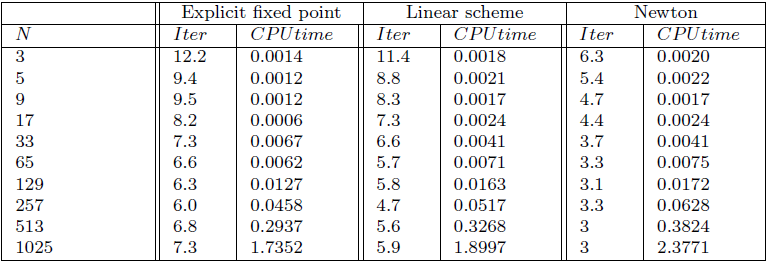
Rmk. Explicit fixed point performs the best in terms of CPU time

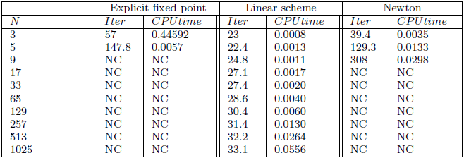
Heisenberg spin chain

Spatial semidiscretization of the Landau–Lifshitz–Gilbert Hamiltonian PDE, $\sigma_t:S^1\rightarrow S^2$

$\dot{\sigma}=\sigma\times\partial_{xx}\sigma$

Give the Hamiltonian isospectral flow on $\mathfrak{su}(2)^{\oplus_N}$, for $N\geq 1$

$\dot{S}_i=[S_i,S_{i-1}+S_{i+1}]$

for $i=1,...,N$ with $S_1\equiv S_N$

Time-step $h=0.5$, normalized initial data

Rmk. Explicit fixed point performs the best in terms of stabilty and CPU time. 

Heisenberg spin chain

An unpractical scheme

Quadratic iteration

• The first equation is CARE (Continuous Algebraic Riccati Equation) in $P_k$
  
  
   
• Non-uniqueness issues

Quadratic iteration
 non-uniqueness issues

Prop. Let $A,B\in\mathfrak{su}(N)$ be non-singular, with signature matrix equal to $I_{p,N-p}$.

Then, the equation $ZAZ^*=B$ has solution $Z\in GL(N,\mathbb{C})$  if and only if $Z=C U D$, for some $U\in U(p,N-p)$ and $C,D$ non-singular such that $B = C I_{p,N-p} C^*$ and $DA D^*=  I_{p,N-p}$. 

Ex. Search for $Z=I + P$, for $P$ skew-Hermitian.

Let $A,B$ diagonal s.t. $i(A-B)\geq 0$.

Then, any $P$ diagonal skew-hermitian (i.e. purely imaginary) such that $P^2=BA^{-1}-I$ is a solution.
For generic $A,B$ as above, we get $2^N$ solutions.

Conclusions

Conclusions

• Iterative schemes for the solution of cubic matrix equations arising in the numerical solution of certain conservative PDEs
• Geometrical integrators: preservation of important physical features
• Both fixed point iterations and inexact Newton work well
• Fixed point iterations more efficient for large time-step and large dimensions
• Implicit fixed point iteration is more stable

Thanks for your attention