Milo Viviani 
(joint work with Francesco Grotto and Marco Romito)

Scuola Normale Superiore - Pisa

YoungStats Webinar - Stochastic fluid dynamics
15 November 2023

2D Euler Equations

Vorticity formulation

• \(\omega\) is the scalar vorticity field \(\omega=\nabla\times u\)
• \(\psi\) is the stream function
• The spatial domain is \(\mathbb{R}^2\)
• Global well posedness for \(\omega_0\in L^1(\mathbb{R}^2)\cap L^\infty(\mathbb{R}^2)\)

Point-vortex Equations

• \(x_i\) are the positions of the vortices
• \(\Gamma_i\) are the intensities of the vortices
• Well-posed for almost any initial configuration, w.r.t. the Lebesgue measure [Marchioro&Pulvirenti, 1994]
• The initial positions \(x_i(0)\) for which the vortices collapse is dense in \(\mathbb{R}^{2N}\), for \(N>2\)

for \(i=1,2,\dots,N\)

Point-vortex as solutions to the 2D Euler Equations

• Solves the Euler equations in the sense of distributions if the self-interaction terms are neglected [Schochet, 1996]
• Point-vortex equations can be obtained as limit of smooth solutions to the Euler equations
• Point-vortex solutions for a finite dimensional coadjoint orbit in \(\Xi_{vol}^*\) [Marsden&Weinstein, 1983]

Empirical measure

Continuation after collapse

Deterministic [Godota&Sakajo, 2016]

for \(i=1,2,\dots,N\)

where, for any \(\varepsilon>0\), \(K_\varepsilon = \varrho^\varepsilon\ast K\), \(K(x) = \frac{x^\perp}{|x|^2}\),

for \(\varrho:\mathbb{R}\rightarrow\mathbb{R}\) convolution kernel \(\varrho^\varepsilon(x) = \frac{1}{\varepsilon^2}\varrho(\frac{x}{\varepsilon})\) 

Given \(x_1(0), x_2(0), x_3(0)\) collapsing intial configuration, for \(\varepsilon\rightarrow 0\)

• \(x_i^\varepsilon(t)\rightarrow x_i(t)\) for \(t\in[0,t_c]\)
• \(x_i^\varepsilon(t)\rightarrow \overline{x}_i(2t_c-t)\) for \(t\in[t_c,2t_c]\)

where \(\overline{x}_i=(x_{i,1},-x_{i,2})\)

Continuation after collapse

Stochastic [Flandoli&Gubinelli&Priola, 2011]

for \(i=1,2,\dots,N\)

where, for any \(\varepsilon>0\), \(B^i\) are i.i.d. 2D Brownian motions. Implies pathwise unique strong solution for \(t\geq 0\).

Given \(x_1(0)^\varepsilon, x_2(0)^\varepsilon, x_3(0)^\varepsilon\) collapsing intial configuration, for \(\varepsilon\rightarrow 0\)

• \(Law(x_1^\varepsilon,x_2^\varepsilon,x_3^\varepsilon)\Rightarrow Law(x_1,x_2,x_3)\), for \(\varepsilon\rightarrow 0\) in \(t\in[0,2t_c]\), up to subsequences 
• Pathwise convergence before \(t_c\) but not after

OPEN QUESTION: What is the limit \(Law(x_1,x_2,x_3)\)?

First integrals in \(\mathbb{R}^2\)

The Point-vortex equations in \(\mathbb{R}^2\) admit the following first integrals

• Energy: \(H=-\frac{1}{2\pi}\sum_{i\neq j} \Gamma_i\Gamma_j \log|x_i-x_j|\)
• Barycenter: \(M=\sum_{i\neq j} \Gamma_ix_i\)
• Moment of intertia: \(I =\sum_{i\neq j} \Gamma_i\Gamma_j|x_i-x_j|^2\)

For N=3, the point-vortex equations exhibit (self similar) collapse in finite time if and only if

• \(\sum_{i\neq j} \Gamma_i\Gamma_j = 0\)
• \(I=\sum_{i\neq j} \Gamma_i\Gamma_j|x_i-x_j|^2 = 0\)

Reduced equations

• For N=3, given a collapsing initial configuration with \(M=0\), by invariance under rotation and homotheties of the collapsing condition, we can study \(Rx_1\), such that
  \(Rx_3=(1,0)\) and \(\Gamma_2Rx_2=-\Gamma_3Rx_3 -\Gamma_1Rx_1\), for a suitable matrix \(R\in O(2)^+\)
   
• Let \(Z:=Rx_1\)We then have \(H=H(Z)\) and \(I = I(Z)\)
• We study how \(H\) and \(I\) change after the collapse for \(\varepsilon\rightarrow 0\)
• The set \(\lbrace Z\in\mathbb{R}^2:H(Z)=H_0\cap I(Z)=I_0\rbrace\) determines the possible configurations

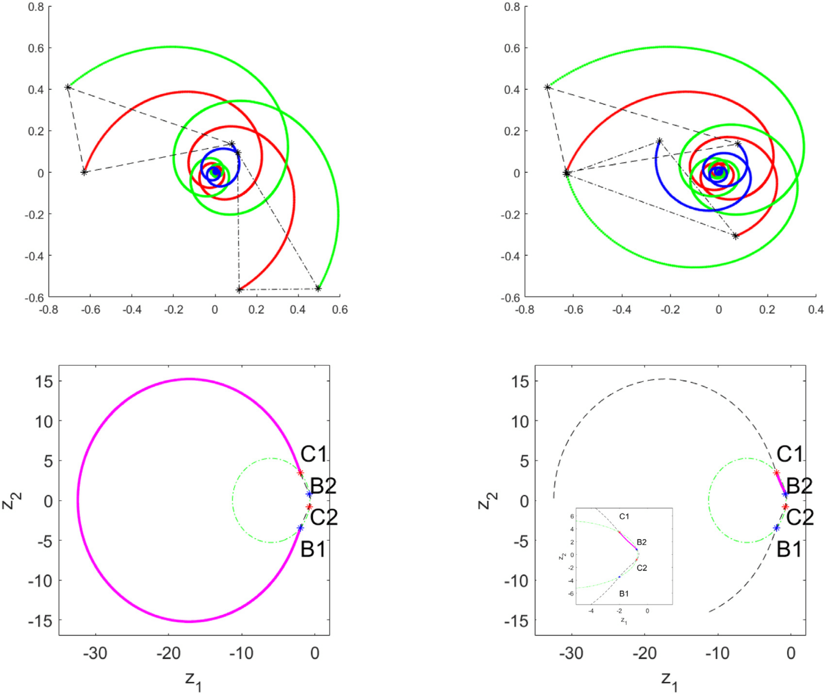
Numerical simulations

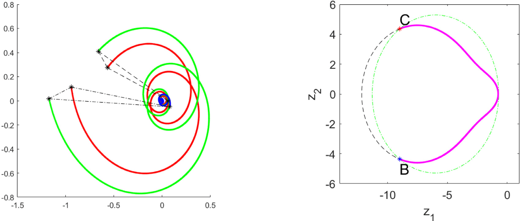
Trajectories \(x^\varepsilon_1,x^\varepsilon_2,x^\varepsilon_3\)

Evolution of \(Z(t)\) purple, green \(I=I_0\), black \(H=H_0\)

\(\varepsilon = 10^{-10}\)

Rmk: \(H\) and \(I\) are local martingales

Numerical scheme

• Adaptive symplectic integrator (midpoint scheme)
• Stochastic midpoint [Burrage&Burrage, 2014], two evaluations of the Wiener process 

where the time-step \(h:=h(n)\) is such that \(h(n)\sigma(x^n_1,x^n_2,x^n_3)^\alpha=h(0)\sigma(x^0_1,x^0_2,x^0_3)^\alpha\), for \(\alpha=1.3\) and \( \sigma(x_1,x_2,x_3)=\frac{1}{\frac{1}{\|x_1-x_2\|^2}+\frac{1}{\|x_2-x_3\|^2}+\frac{1}{\|x_1-x_3\|^2}}\)

Statistics for the limiting distribution

• Evidences of non-uniform distribution of the reopening angle \(\theta\), defined as the angle between \(x_2^\varepsilon\) and the \(x-\)axis at \(t=2t_c\), for \(\varepsilon\rightarrow 0\):
  - strong fluctuations of CDF for different \(\varepsilon\) may indicate non-unique limit distribution;
  - p-values\(<<10^{-9}\), for \(\varepsilon=10^{-10}\), tested on the uniform distribution hypotesis for \(\theta\)
   
• Evidences of equal probability in keeping or changing configuration after collapse (4 intersections of \(H\) and \(I\)), p-value=0.295, for \(\varepsilon=10^{-10}\)

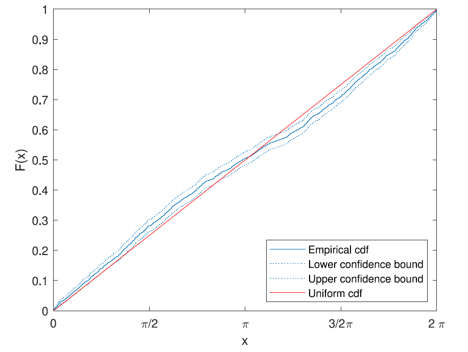
Empirical c.d.f. (solid blue) of the angle of \(x_2^\varepsilon(2t_c)\) for \(10^4\) samples, \(\varepsilon=10^{-10}\) . Dotted blue curves are confidence bounds (\(95\%\)) for the e.c.d.f. and the solid red line is the c.d.f. of the uniform distribution on \([0,2\pi]\).

Empirical CDF

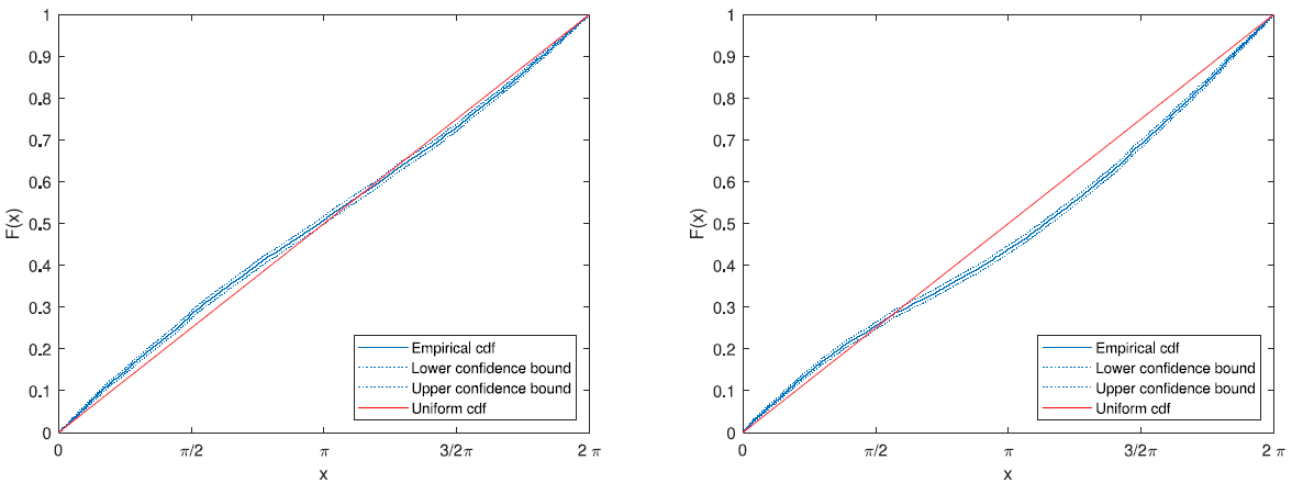
Empirical c.d.f. (solid blue) of the angle of \(x_2^\varepsilon(2t_c)\) for \(10^4\) samples, \(\varepsilon=10^{-10}\) . Dotted blue curves are confidence bounds (\(95\%\)) for the e.c.d.f. and the solid red line is the c.d.f. of the uniform distribution on \([0,2\pi]\). Samples being divided (right and left plots) according to the similarity class of the PV position triangle during burst.

Empirical CDF