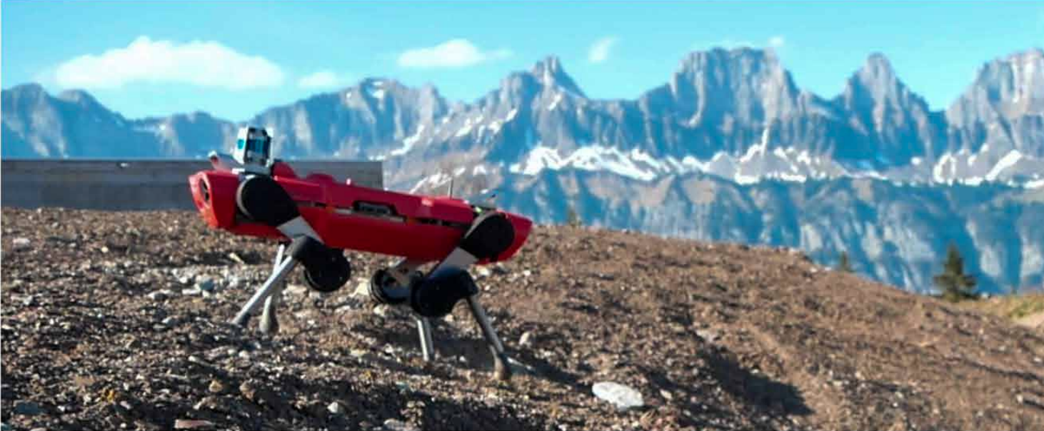
Planning and Control for Contact-rich Manipulation
Tao Pang
Oct 2022
Why contact-rich?
Collision-free Motion Planning
Interact with the world
Interact with the world
Collision-free Motion Planning
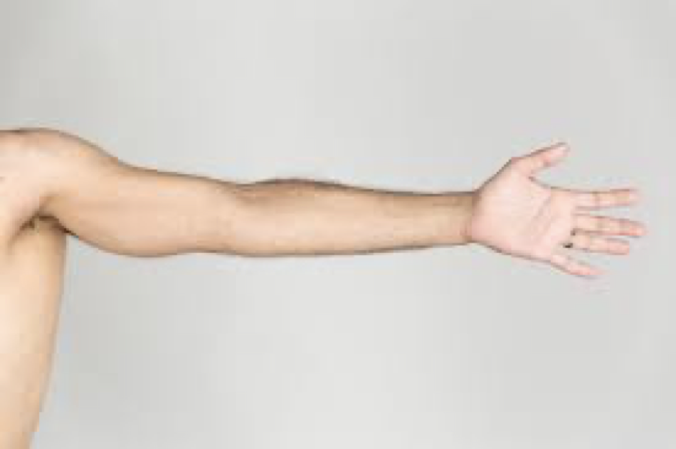
But this is excessively restrictive!
We'd like to enable robots to make contacts with the world like humans do.
Why contact-rich?
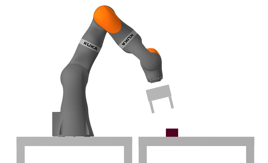
Box
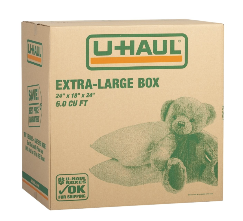
What if we have a larger box...?
We need to use a bigger arm...
Or make more contacts!
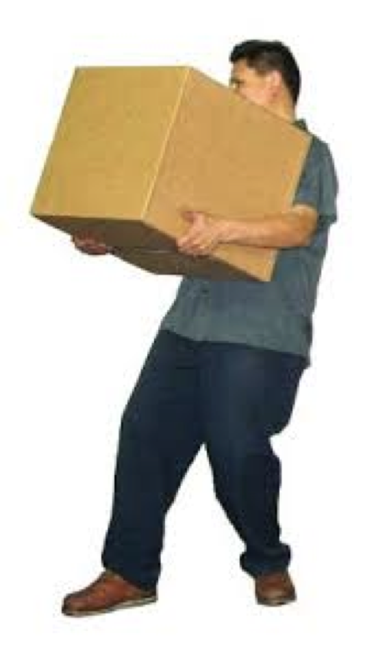
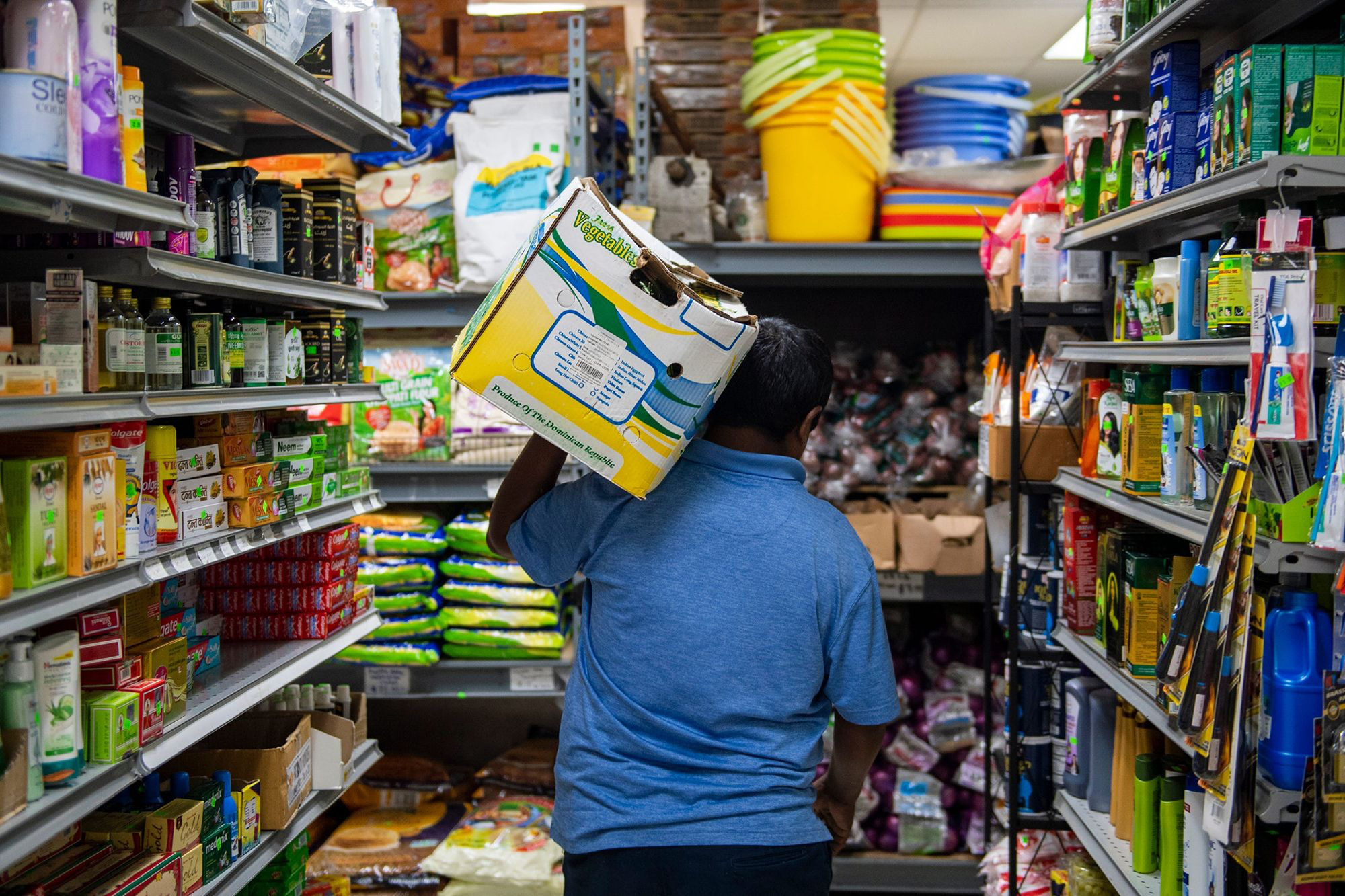
- Contact-rich manipulation allows smaller robots to handle bigger objects.
- Smaller robots are safer to easier to work in environments designed for humans.
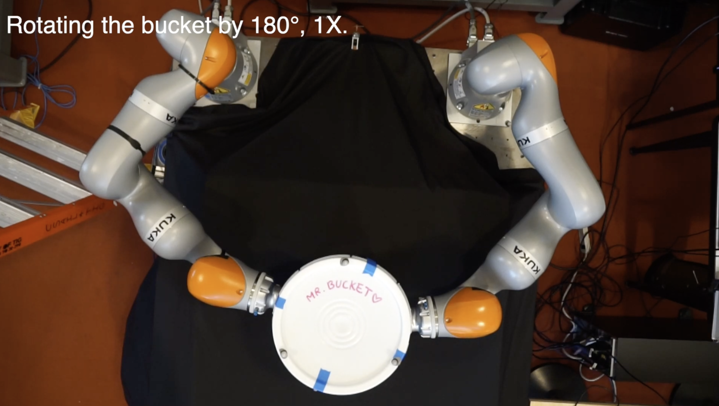
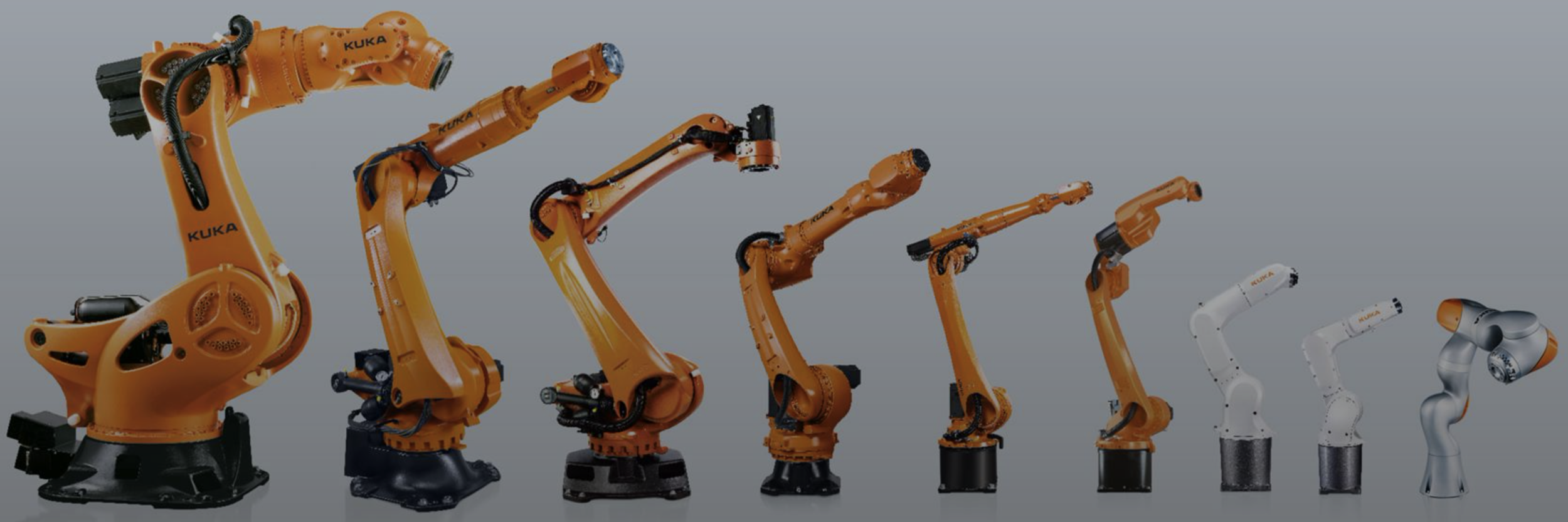
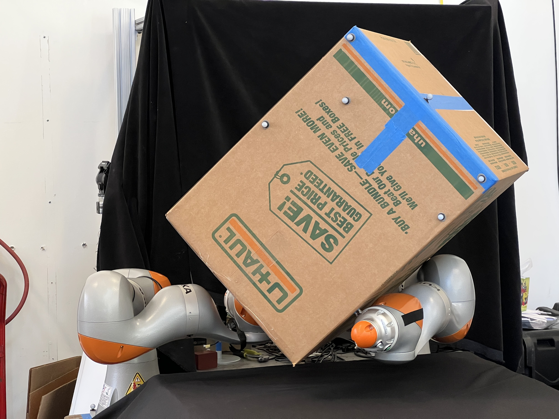
Contact-rich Manipulation at Different Scales
A few more arms
Smaller
Contact-rich planning and control can enable both bimanual whole-arm manipulation and dexterous manipulation.
Why is contact-rich planning hard?
Contact dynamics is non-smooth!
Two solutions
Smooth contact-dynamics and use smoothed gradients
Reason explicitly about contact mode transitions
q^\mathrm{a}_+
u
Contact
No Contact
- But descent methods get stuck in local minima.
- Good at escaping local minima,
- But mode enumeration scales poorly (exponentially) with the number of contacts.
x_+ = u
x_+ = 0
u > 0
u \leq 0
q^\mathrm{a}_+
u
smoothed dynamics
original dynamics
\(u = 0\)
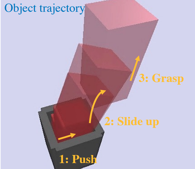
Model-based Planning through Contact: a Quick Review
- Trajectory Optimization through Contact
- Mordatch, Igor, Emanuel Todorov, and Zoran Popović. "Discovery of complex behaviors through contact-invariant optimization." ACM Transactions on Graphics (TOG), 2012.
- Hogan, François Robert, and Alberto Rodriguez. "Feedback control of the pusher-slider system: A story of hybrid and underactuated contact dynamics." arXiv preprint arXiv:1611.08268 (2016).
- Posa, Michael, Cecilia Cantu, and Russ Tedrake. "A direct method for trajectory optimization of rigid bodies through contact." The International Journal of Robotics Research, 2014.
- Aydinoglu, Alp, and Michael Posa. "Real-time multi-contact model predictive control via admm." 2022 International Conference on Robotics and Automation (ICRA), 2022.
- Cheng, Xianyi, et al. "Contact mode guided motion planning for quasidynamic dexterous manipulation in 3d." 2022 International Conference on Robotics and Automation (ICRA), 2022.
- Marcucci, Tobia, et al. "Approximate hybrid model predictive control for multi-contact push recovery in complex environments." 2017 IEEE-RAS 17th International Conference on Humanoid Robotics (Humanoids), 2017.
- Enumerate mode switches locally
- Enumerate Mode Switches
- Sampling mode switches
Smoothed Contact Dynamics
Hybrid Contact Dynamics
Local Planning
Global Planning
Smoothed dynamics + Global planning?
[1] Mordatch et al.

[3] Posa et al.
[5] Cheng et al.
[6] Marcucci et al.
[4] Aydinoglu and Posa.

[2] Hogan and Rogriguez.
What about RL (reinforcement learning)?
- RL generates robust policies for specific tasks, but...
- RL requires heavy offline computation,
- the learned policy does not generalize (e.g. to opening a door).
- In contrast, planning can solve new tasks with a small amount of online compute.
- We believe a good manipulation pipeline will have both plans and policies.
- Andrychowicz, OpenAI: Marcin, et al. "Learning dexterous in-hand manipulation." The International Journal of Robotics Research, 2020.
- Lee, Joonho, et al. "Learning quadrupedal locomotion over challenging terrain." Science robotics, 2020.
-
H.J. Terry Suh*, Tao Pang*, Russ Tedrake, “Bundled Gradients through Contact via Randomized Smoothing”, RA-L, 2022.
-
Tao Pang*, H.J. Terry Suh*, Lujie Yang, Russ Tedrake, "Global Planning for Contact-Rich Manipulation via Local Smoothing of Quasi-dynamic Contact Models", under review.
[2] Lee et al.
[1] OpenAI.
How does RL power through non-smooth contact dynamics? [3][4]
- RL minimizes a stochastic objective via sampling.
- Sampling has a smoothing effect on the objective's landscape.
Taking a page from RL's book, we smooth contact dynamics, but without using samples (faster).
Terry Suh
Why is contact-rich planning hard?
Contact dynamics is non-smooth!
q^\mathrm{a}_+
u
Contact
No Contact
\begin{aligned}
\underset{q^\mathrm{a}_+}{\min.} \; &\frac{1}{2} (q^\mathrm{a}_+ - u)^2, \text{s.t.} \\
&q^\mathrm{a}_+ \geq 0
\end{aligned}
\begin{aligned}
\underset{q^\mathrm{a}_+}{\min.} \; &\frac{1}{2} (q^\mathrm{a}_+ - u)^2 - \frac{1}{\kappa} \mathrm{log}(q^\mathrm{a}_+)
\end{aligned}
Smoothing
Our method: Kino-dynamic RRT through contact
- We leverage the sampling-based nature of RRT to globally explore the state space.
- Instead of thinking about mode transitions, we abstract modes away using smoothed linearization of the contact dynamics.
- We propose an reachability-based distance metric for RRT to efficiently explore the state space.
- Mode abstraction and the distance metric are enabled by a Convex, Quasi-static, Differentiable contact dynamics model.
- Convex: the discrete-time dynamics \(x_+ = f(x, u)\) can be evaluated by solving a convex program.
-
Quasi-static:
- Valid for many manipulation tasks.
- Smaller state space,
- Larger step size,
- The dynamics model can be easily smoothed.
- Differentiable: the smoothed gradients can help RRT by providing an effective distance metric.
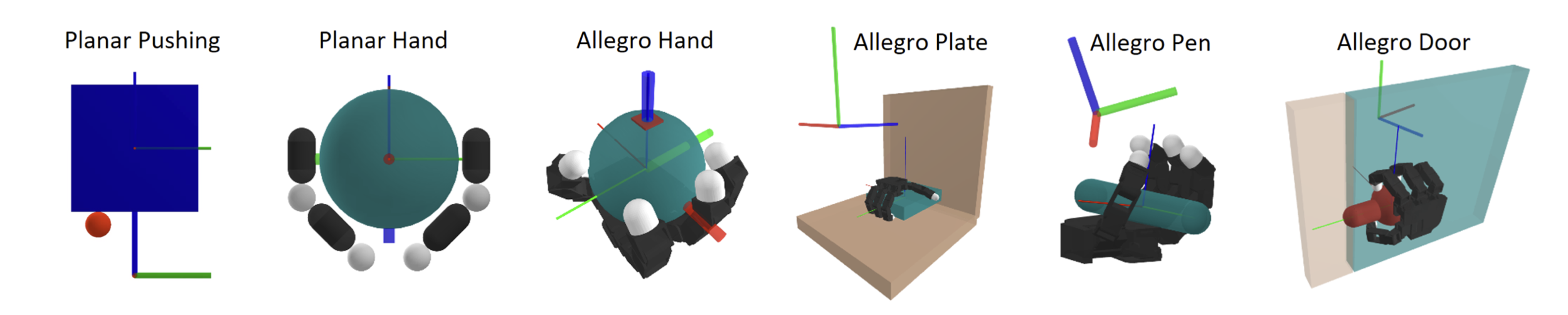
Our Method: Sim and Hardware Demos.
- RRT takes less than a minute.
Open-loop execution of contact-rich plans:
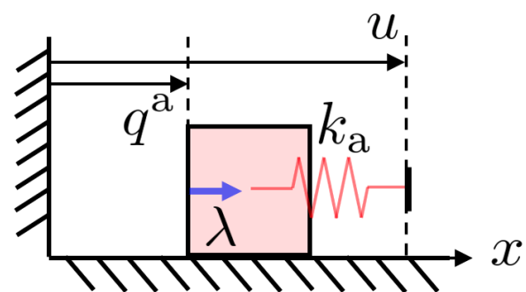
What is quasi-static dynamics?
q^\mathrm{a}
u
K_\mathrm{a}
q^\mathrm{u}
- Quasi-static: velocity is small so that inertial and Coriolis forces are negligible.
- \(x \coloneqq q \coloneqq [q^\mathrm{u}, q^\mathrm{a}]\): system configuration.
- \(q^\mathrm{a}\): actuated, imepdance-controlled robots
- \(q^\mathrm{u}\): un-actuated objects.
- \( u \):
robot velocitiesposition command to the stiffness-controlled robots [1]. - \(\delta q \coloneqq q_+ - q\)
- \(h\): step size in seconds.
\( x_{+} = f(x, u)\)
\lambda_1
\lambda_3
\lambda_1
\lambda_2
- \(\lambda_i\): contact forces/impulses
- \(\phi_i \): signed distances
\phi_2({q})
\phi_1({q})
\phi_3({q})
\begin{aligned}
\underset{\delta q^\mathrm{a}, \delta q^\mathrm{u}}{\min} \; &\frac{1}{2} hK (q^\mathrm{a} + \delta q^\mathrm{a} - u)^2 \; \text{s.t.} \\
&\phi_i (q + \delta q)\geq 0, \forall i.
\end{aligned}
\Leftrightarrow
(KKT)
- A convex quadratic program (QP), after linearizing \(\phi_i\).
- "Minimizing potential energy, subject to non-penetration constraints."
\begin{cases}
hK(q^\mathrm{a} + \delta q^\mathrm{a} - u) = -\lambda_1 + \lambda_2, \\
0 = \lambda_1 - \lambda_3, \\
\phi_i(q + \delta q) \geq 0, \; \forall i, \\
\lambda_i \geq 0 \; \forall i, \\
\phi (q + \delta q) \lambda = 0, \forall i.
\end{cases}
Force balance of the robot.
Force balance of the object.
Non-penetration.
"Contact forces cannot pull."
"Contact force needs contact."
-
Tao Pang, Russ Tedrake, "A Convex Quasistatic Time-stepping Scheme for Rigid Multibody Systems with Contact and Friction", ICRA, 2021.
Quasi-static dynamics is good for manipulation planning!
- Many manipulation tasks are quasi-static.
- Spatial benefit: Smaller state space (\([q, v]\) vs. only \(q\)).
-
Temporal benefit: Ignoring transients => looking into the future with fewer steps.
-
Tao Pang, Russ Tedrake, "A Convex Quasistatic Time-stepping Scheme for Rigid Multibody Systems with Contact and Friction", ICRA, 2021.
q^\mathrm{a}
m^\mathrm{a}
u
K
D
Second-order Dynamics
Quasi-static Dynamics
\begin{aligned}
m^\mathrm{a} &= 1.0 \\
D &= 20.0\\
K &= 100.0
\end{aligned}
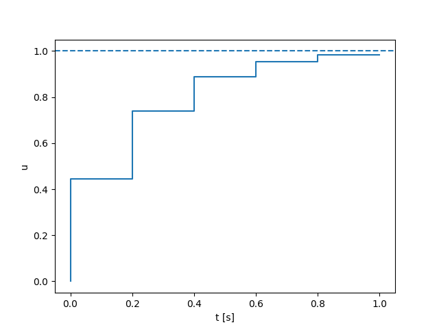
Quasi-static Dynamics Needs Regularization
\begin{aligned}
\underset{\delta q^\mathrm{a}, \delta q^\mathrm{u}}{\min} \; &\frac{1}{2} hK (q + \delta q^\mathrm{a} - u)^2, \; \text{s.t.} \\
&\phi_i (q + \delta q)\geq 0, \forall i.
\end{aligned}
Quasi-static Dynamics
- The quadratic cost is positive semi-definite.
- The object can be anywhere between the robot and the wall, similar to having a null space.
\underset{x}{\min} \|Ax - b\|^2
\underset{x}{\min} \|Ax - b\|^2 + \epsilon \|x\|^2
Regularized least squares
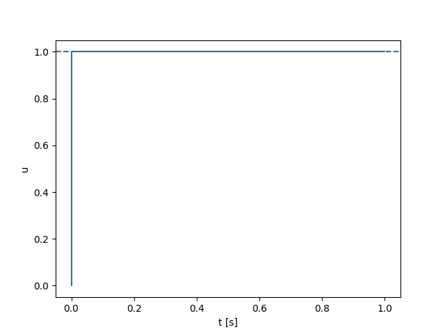
Regularized Quasi-static Dynamics
\begin{aligned}
\underset{\delta q^\mathrm{a}, \delta q^\mathrm{u}}{\min} \; &\frac{1}{2} hK (q^\mathrm{a} + \delta q^\mathrm{a} - u)^2 + \frac{1}{2} \epsilon (\delta q^\mathrm{u})^2, \; \text{s.t.} \\
&\phi_i (q + \delta q)\geq 0, \forall i.
\end{aligned}
- The quadratic cost is now positive definite.
- "Among all possible object motions, give me the one that moves the least."
- Picking \(\epsilon = m^\mathrm{u} / h\) gives Mason's definition of quasi-dynamic dynamics.
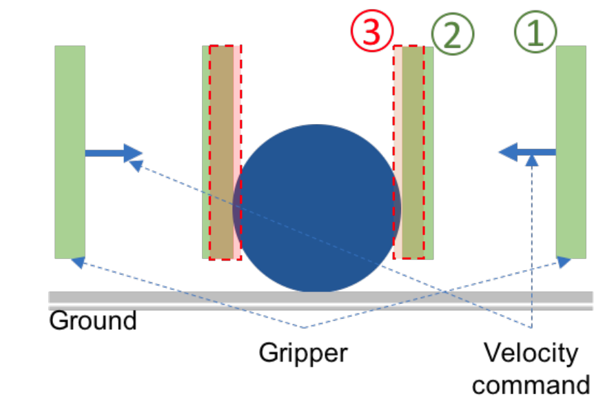
q^\mathrm{a}
u
K_\mathrm{a}
q^\mathrm{u}
\phi_2({q})
\phi_1({q})
\phi_3({q})
What about friction?
\begin{aligned}
\underset{\delta q}{\min} \;
&\frac{1}{2}
{\underbrace{
\begin{bmatrix}
\delta q^\mathrm{u} \\
\delta q^\mathrm{a}
\end{bmatrix}}_{\delta q}}^\intercal
\underbrace{
\begin{bmatrix}
\mathbf{M}_\mathrm{u} / h & 0 \\
0 & h \mathbf{K}_\mathrm{a}
\end{bmatrix}}_{\mathbf{Q}}
\underbrace{
\begin{bmatrix}
\delta q^\mathrm{u} \\
\delta q^\mathrm{a}
\end{bmatrix}}_{\delta q}
+
{\underbrace{
h
\begin{bmatrix}
- \tau^\mathrm{u} \\
- \mathbf{K}_\mathrm{a} (u - q^\mathrm{a}) - \tau^\mathrm{a}
\end{bmatrix}}_{b}}^\intercal
\underbrace{
\begin{bmatrix}
\delta q^\mathrm{u} \\
\delta q^\mathrm{a}
\end{bmatrix}}_{\delta q}
\;\text{s.t.} \\
&\underbrace{\phi_i + \mathbf{J}_{\mathrm{n}_i}\delta q}_{\text{Linearized} \; \phi_i(q + \delta q)} \geq 0, \; \forall i \in \{1 \cdots n_{\mathrm{c}}\}.
\end{aligned}
- For a frictionless multi-body system with \(n_\mathrm{c}\) contacts, the dynamics can be solved as a QP:
- \(\mathcal{K}^\star_i\) is the dual of the \(i\)-th friction cone.
- Still convex! Convexity is achieved at the expense of "hydroplaning" between relatively-sliding objects.
- But hydroplaning disappears as \(h \rightarrow 0\).
\begin{aligned}
\underset{\delta q}{\min} \;
&\frac{1}{2} {\delta q}^\intercal \mathbf{Q} \delta q + b^\intercal \delta q \;\text{s.t.} \\
&
\begin{bmatrix}
\phi_i + \mathbf{J}_{\mathrm{n}_i}\delta q \\
\mathbf{J}_{\mathrm{t}_i}\delta q
\end{bmatrix}
\in \mathcal{K}^\star_i, \; \forall i \in \{1 \cdots n_{\mathrm{c}}\}.
\end{aligned}
- Anitescu [1] has a nice convex approximation of Coulomb friction constraints, allowing us to write down the dynamics as a Second-Order Cone Program (SOCP):
Tangential displacements
\begin{aligned}
\underset{\delta q^\mathrm{a}, \delta q^\mathrm{u}}{\min} \; &\frac{1}{2} hK (q + \delta q^\mathrm{a} - u)^2 + \frac{1}{2} \frac{m^\mathrm{u}}{h} (\delta q^\mathrm{u})^2, \; \text{s.t.} \\
&\phi_i (q + \delta q)\geq 0, \; \forall i.
\end{aligned}
Dynamics of the Toy Problem
- Anitescu, Mihai. "Optimization-based simulation of nonsmooth rigid multibody dynamics." Mathematical Programming 105.1 (2006): 113-143.
Differentiability
\begin{aligned}
\delta q^\star \coloneqq \underset{\delta q}{\text{argmin}.} \;
&\frac{1}{2} {\delta q}^\intercal \mathbf{Q} \delta q + b^\intercal \delta q \;\text{s.t.} \\
&
\begin{bmatrix}
\phi_i + \mathbf{J}_{\mathrm{n}_i}\delta q \\
\mathbf{J}_{\mathrm{t}_i}\delta q
\end{bmatrix}
\in \mathcal{K}^\star_i, \; \forall i \in \{1 \cdots n_{\mathrm{c}}\}.
\end{aligned}
Convex, Quasi-Static, Differentiable Dynamics (an SOCP)
q_+ = f(q, u) = q + \delta q^\star(q, u)
\newcommand{\DfDx}[2]{\frac{\partial {#1}}{\partial {#2}}}
\mathbf{A} \coloneqq \DfDx{f}{q} = \mathbf{I} + \DfDx{\delta q^\star}{q}, \;
\mathbf{B} \coloneqq \DfDx{f}{u} = \DfDx{\delta q^\star}{u},
- The KKT optimality condition of the dynamics SOCP defines equality constraints (including active contact constraints), from which the derivatives of \(\delta q^\star\) w.r.t. \((\mathbf{Q}, b, \phi_i, \mathbf{J}_{\mathrm{n}_i}, \mathbf{J}_{\mathrm{t}_i})\) can be computed using the Implicit Function Theorem (IFT).
- \(\mathbf{A}, \mathbf{B}\) can then be computed using the gradients from IFT and the chain rule.
- Standard practice for many differentiable simulators, even though many of them do not find the active constraints by solving convex programs.
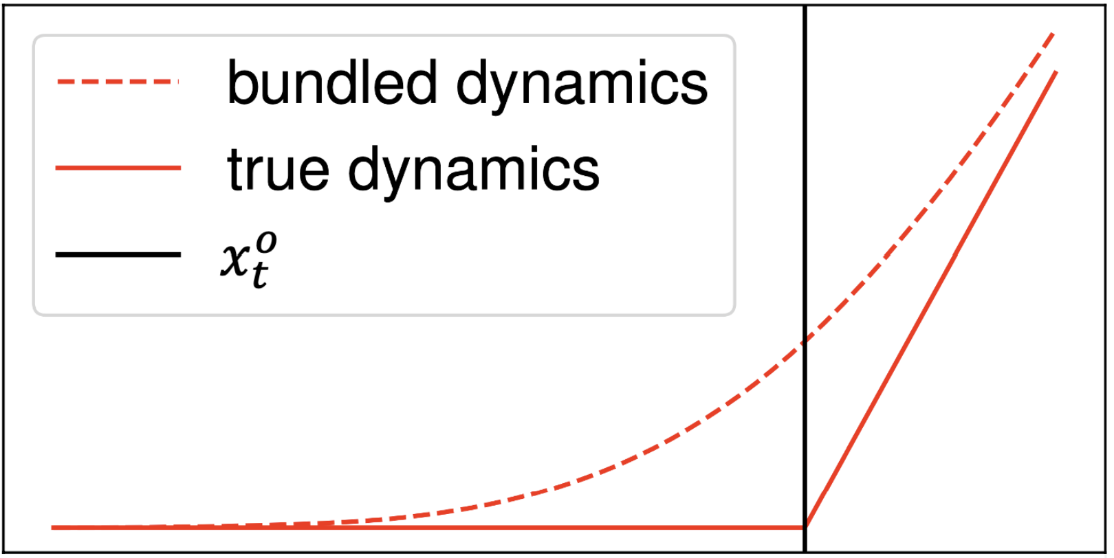
Smoothing
- The contact dynamics \(f(q, u) \in C^0\) has discontinuous gradients, which are bad for planning methods that use gradients.
- Smoothing with "force at a distance" is a common method to alleviate this problem.
Optimality Condition
\begin{aligned}
\underset{\delta q^\mathrm{a}, \delta q^\mathrm{u}}{\min} \; &\frac{1}{2} hK (q + \delta q^\mathrm{a} - u)^2 + \frac{1}{2} \frac{m^\mathrm{u}}{h} (\delta q^\mathrm{u})^2
- \frac{1}{\kappa}\sum_i\log{\phi_i(q + \delta q)}
\end{aligned}
\Leftrightarrow
\begin{aligned}
\underset{\delta q^\mathrm{a}, \delta q^\mathrm{u}}{\min} \; &\frac{1}{2} hK (q + \delta q^\mathrm{a} - u)^2 + \frac{1}{2} \frac{m^\mathrm{u}}{h} (\delta q^\mathrm{u})^2, \; \text{s.t.} \\
&\phi_i (q + \delta q)\geq 0, \forall i.
\end{aligned}
\Leftrightarrow
KKT
Original Dynamics
\begin{cases}
hK(q^\mathrm{a} + \delta q^\mathrm{a} - u) = -\lambda_1 + \lambda_2, \\
(m^\mathrm{u} / h) \delta q^\mathrm{u} = \lambda_1 - \lambda_3, \\
\phi_i(q + \delta q) \geq 0, \; \forall i, \\
\lambda_i \geq 0, \; \forall i, \\
\phi (q + \delta q) \lambda = 0, \forall i.
\end{cases}
q^\mathrm{a}
u
K_\mathrm{a}
q^\mathrm{u}
\lambda_1
\lambda_3
\lambda_1
\lambda_2
\phi_2({q})
\phi_1({q})
\phi_3({q})
Smoothed Dynamics
\begin{cases}
hK(q^\mathrm{a} + \delta q^\mathrm{a} - u) = -\lambda_1 + \lambda_2, \\
(m^\mathrm{u} / h) \delta q^\mathrm{u} = \lambda_1 - \lambda_3, \\
\phi_i(q + \delta q) \geq 0, \; \forall i, \\
\lambda_i \geq 0, \; \forall i, \\
\phi_i (q + \delta q) \lambda = 1 / \kappa, \forall i.
\end{cases}
Smoothing, the general case.
\begin{aligned}
\underset{\delta q}{\text{min}.} \;
&\frac{1}{2} {\delta q}^\intercal \mathbf{Q} \delta q + b^\intercal \delta q \;\text{s.t.} \\
&
\begin{bmatrix}
\phi_i + \mathbf{J}_{\mathrm{n}_i}\delta q \\
\mathbf{J}_{\mathrm{t}_i}\delta q
\end{bmatrix}
\in \mathcal{K}^\star_i, \; \forall i \in \{1 \cdots n_{\mathrm{c}}\}.
\end{aligned}
\underset{\delta q}{\text{min}.} \;
\frac{1}{2} {\delta q}^\intercal \mathbf{Q} \delta q + b^\intercal \delta q
-
\frac{1}{\kappa}
\sum_{i=1}^{n_\mathrm{c}}
\log
\left[
\frac{(\phi_i + \mathbf{J}_{\mathrm{n}_i}\delta q)^2}{\mu_i^2} - (\mathbf{J}_{\mathrm{t}_i}\delta q)^\intercal (\mathbf{J}_{\mathrm{t}_i}\delta q)
\right]
Put constraints in a generalized log for \(\mathcal{\kappa}_i^\star\)
\Rightarrow
- An unconstrained convex program.
- Can be solved with Newton's method.
- Also differentiable.
Convex, Quasi-Dynamic, Differentiable Dynamics (an SOCP)
Notation:
q_+ = f(q, u)
Original dynamics
q_+ = f_\rho(q, u)
Smoothed dynamics
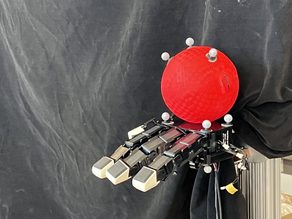
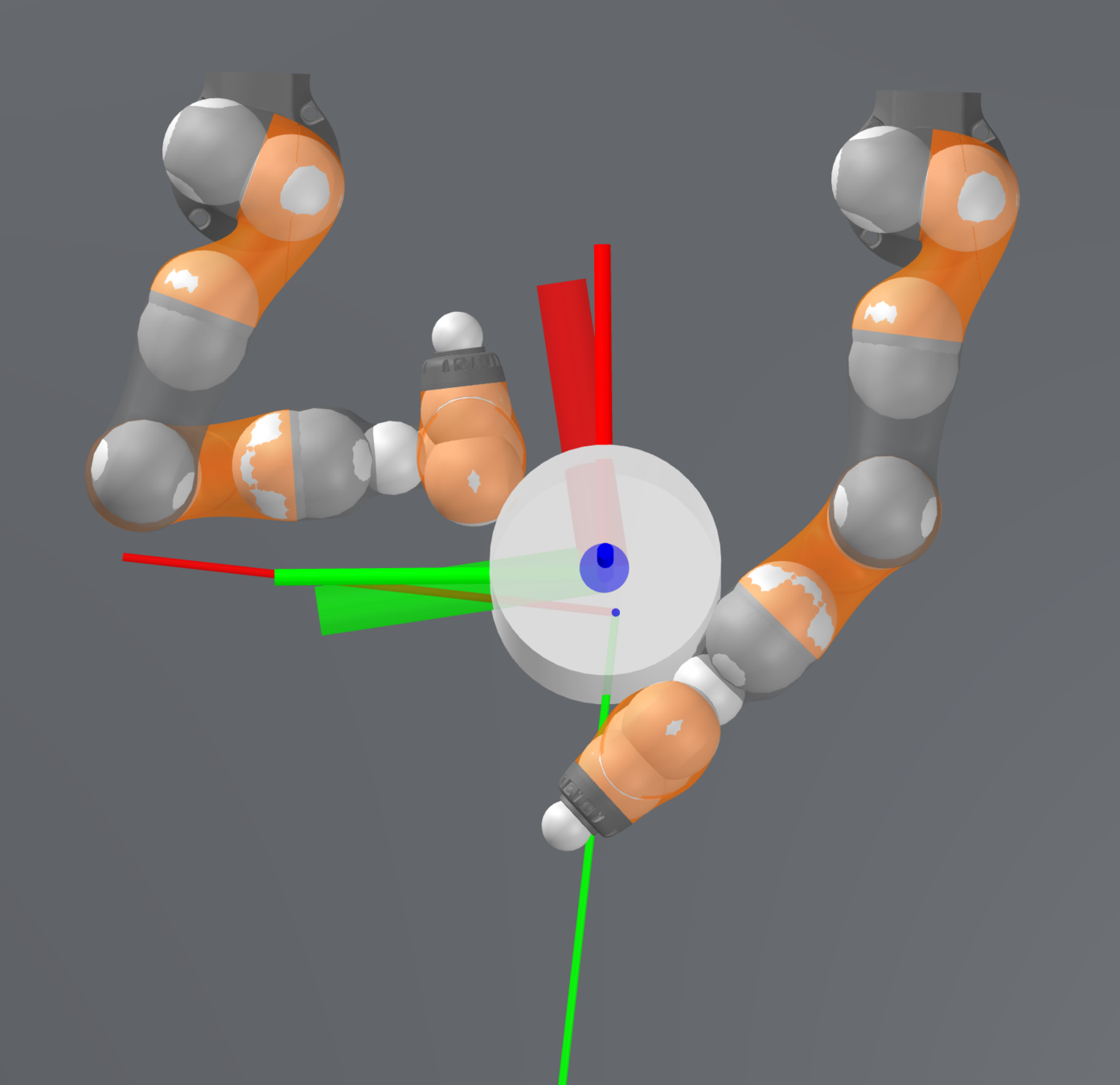
Smoothed gradients enable trajectory optimization for dexterous hands, but...
Task: Turning the ball by 30 degrees.
What about 180 degrees?
Finding this trajectory requires powering through local minima!
Sampling-based Motion Planing is Great at Global Exploration, but...
- Rapidly-Exploring Random Tree (RRT): iteratively builds a tree that fills the state space. [1]
- Dynamic reachability is essential for efficient exploration. [2]
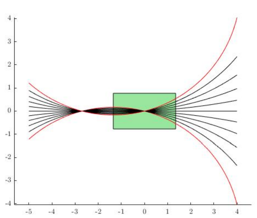
- , "Planning Algorithms", Cambridge University Press , 2006.
-
H.J.T. Suh, J. Deacon, Q. Wang, "A Fast PRM Planner for Car-like Vehicles", self-hosted, 2018.
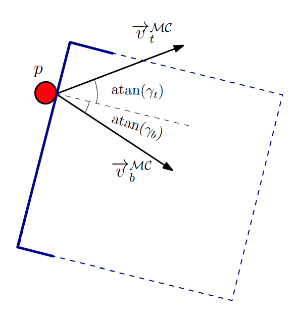
How do we think about reachability under the contact-dynamics constraint?
A distance metric that reflects contact dynamic reachability
q_+ = f_\rho(q, u),
\newcommand{\DfDx}[2]{\frac{\partial {#1}}{\partial {#2}}}
\mathbf{A}_\rho \coloneqq \DfDx{f_\rho}{q}\big|_{q,u}, \\
\mathbf{B}_\rho \coloneqq \DfDx{f_\rho}{u}\big|_{q,u}.
\mathcal{R}_{\rho, \varepsilon}^\mathrm{u} (\bar{q})\coloneqq \left\{\mathbf{B}_\rho^\mathrm{u}(\bar{q},\bar{q}^{\mathrm{a}}) \delta u + f_\rho^\mathrm{u}(\bar{q},\bar{q}^\mathrm{a})\; | \; \|\delta u\|\leq \varepsilon\right\}
Smoothed Contact Dynamics
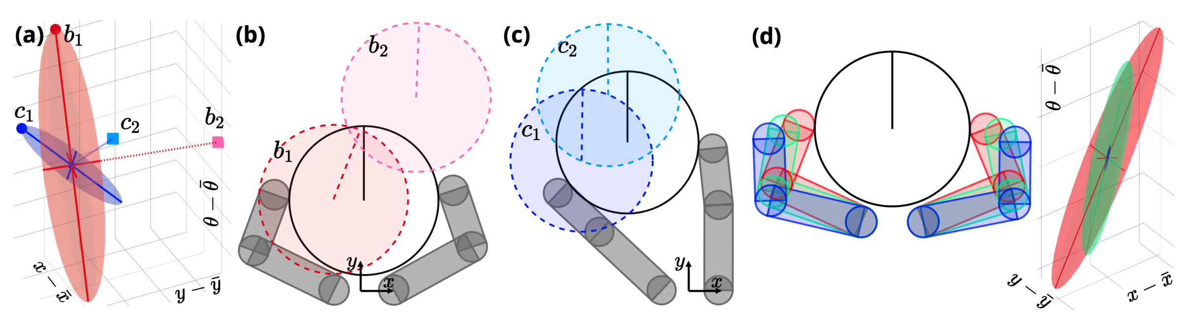
\(\varepsilon \) sub-level set
Nominal state
un-actauted(objects)
Smoothed
\begin{aligned}
d^\mathrm{u}_{\rho}(q; \bar{q}) &\coloneqq \frac{1}{2} (q^\mathrm{u} - \mu^\mathrm{u}_\rho)^\intercal {\left[\mathbf{B}_{\rho}^{\mathrm{u}} {\mathbf{B}_{\rho}^{\mathrm{u}}}^\intercal\right]}^{-1} (q^\mathrm{u} - \mu^\mathrm{u}_\rho) \\
\mu_\rho^\mathrm{u} &\coloneqq f_\rho^\mathrm{u}(\bar{q}, \bar{q}^\mathrm{a})
\end{aligned}
At state \(\bar{q}\), what doe an \(\varepsilon\)-ball in action space get transformed into under the smoothed dynamics?
RRT through contact
Two modifications to the vanilla RRT are made:
- Nearest node on tree is found using \( d^\mathrm{u}_{\rho}(q; \bar{q}) \).
- Contact sampling: robot configuration is occasionally reset to one that has a good distance metric, which typically corresponds to grasps.
Distance Metric
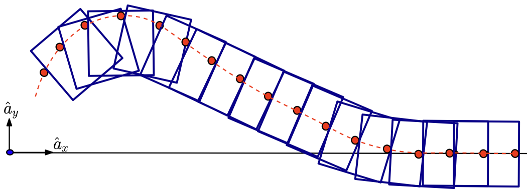
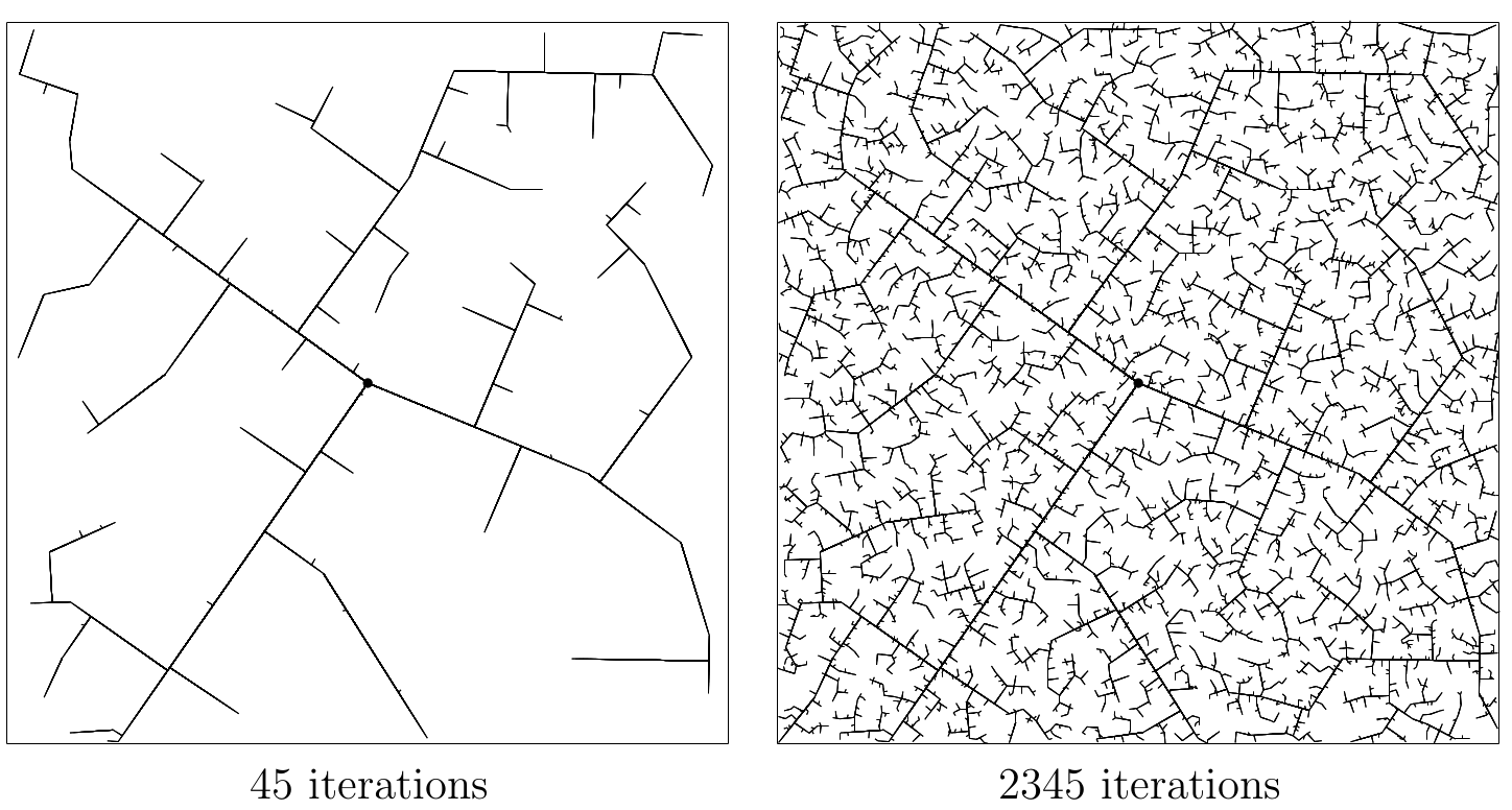
RRT tree for a simple system with contacts
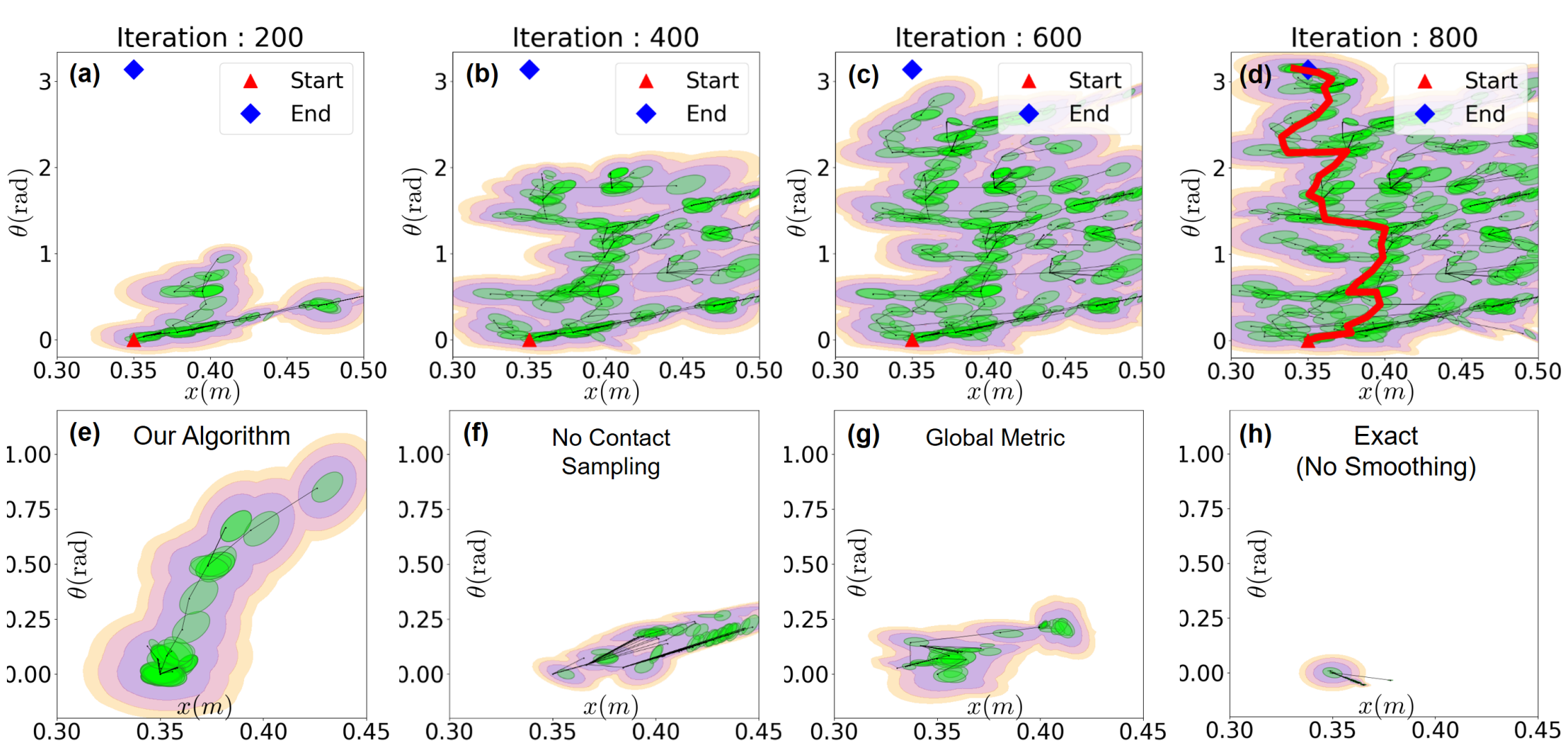
Ablation study: what trees look like after growing a fixed number of nodes.
\begin{aligned}
d^\mathrm{u}_{\rho}(q; \bar{q}) &\coloneqq \frac{1}{2} (q^\mathrm{u} - \mu^\mathrm{u}_\rho)^\intercal {\left[\mathbf{B}_{\rho}^{\mathrm{u}} {\mathbf{B}_{\rho}^{\mathrm{u}}}^\intercal\right]}^{-1} (q^\mathrm{u} - \mu^\mathrm{u}_\rho) \\
\mu_\rho^\mathrm{u} &\coloneqq f_\rho^\mathrm{u}(\bar{q}, \bar{q}^\mathrm{a})
\end{aligned}
The modified RRT works well for contact-rich tasks!
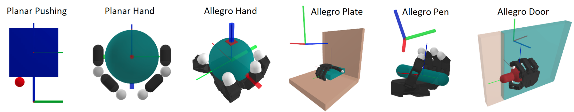
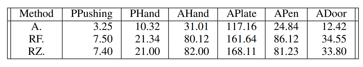
Planning wall-clock time (seconds)
RRT is good at escaping local minima, but...
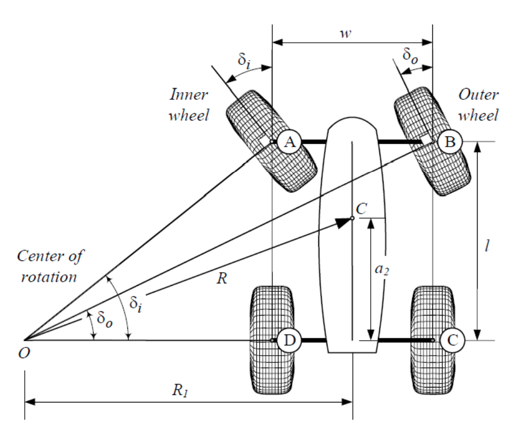
- Kino-dynamic RRT needs a good distance metric! Think about the bycicle.
- A good metric from a queried state \(q\) to a nominal state \(\bar{q}\) can be derived based on the smoothed linearization at \(\bar{q}\):
q_+ = f_\rho(q, u),
\newcommand{\DfDx}[2]{\frac{\partial {#1}}{\partial {#2}}}
\mathbf{A}_\rho \coloneqq \DfDx{f_\rho}{q}\big|_{q,u}, \\
\mathbf{B}_\rho \coloneqq \DfDx{f_\rho}{u}\big|_{q,u}.
\mathcal{R}_{\rho, \varepsilon}^\mathrm{u} (\bar{q})\coloneqq \left\{\mathbf{B}_\rho^\mathrm{u}(\bar{q},\bar{q}^{\mathrm{a}}) \delta u + f_\rho^\mathrm{u}(\bar{q},\bar{q}^\mathrm{a})\; | \; \|\delta u\|\leq \varepsilon\right\}
Smoothed Contact Dynamics
- \(d^\mathrm{u}_{\rho}(q; \bar{q})\) reflects the reachability of \(q\) from \(\bar{q}\) under the smoothed linearization.
\begin{aligned}
d^\mathrm{u}_{\rho}(q; \bar{q}) &\coloneqq \frac{1}{2} (q^\mathrm{u} - \mu^\mathrm{u}_\rho)^\intercal {\left[\mathbf{B}_{\rho}^{\mathrm{u}} {\mathbf{B}_{\rho}^{\mathrm{u}}}^\intercal\right]}^{-1} (q^\mathrm{u} - \mu^\mathrm{u}_\rho) \\
\mu_\rho^\mathrm{u} &\coloneqq f_\rho^\mathrm{u}(\bar{q}, \bar{q}^\mathrm{a})
\end{aligned}
\(\varepsilon \) sub-level set
\begin{aligned}
q_+ &= \mathbf{B}_\rho (u - \bar{u}) + f_\rho(\bar{q}, \bar{u}) \\
\mathbf{B}_\rho &= \frac{\partial f_\rho}{\partial u}\Big|_{\bar{q}, \bar{u}}
\end{aligned}
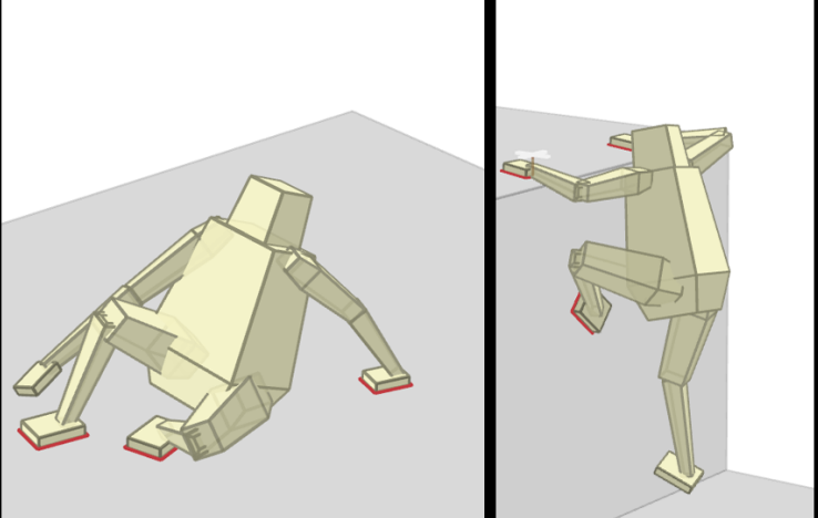
Preliminary: stabilizing contact-rich plans
Open-loop
Closed-loop

\begin{aligned}
\underset{q^\mathrm{u}_+, u}{\min} &\|q_+^\mathrm{u} - q_+^\mathrm{u, ref}\|_\mathbf{Q} + \|u - u^\mathrm{ref} \|_\mathbf{R}, \text{s.t.}\\
& q^\mathrm{u}_+ = f^\mathrm{u}(q^\mathrm{ref}, u^\mathrm{ref}) + \mathbf{B}_\rho^\mathrm{u} (u - u^\mathrm{ref})
\end{aligned}
Naive QP controller based on smoothed linearization:
Presented Works
Collaborators
-
Tao Pang*, H.J. Terry Suh*, Lujie Yang, Russ Tedrake, "Global Planning for Contact-Rich Manipulation via Local Smoothing of Quasi-dynamic Contact Models", under review.
-
H.J. Terry Suh*, Tao Pang*, Russ Tedrake, “Bundled Gradients through Contact via Randomized Smoothing”, RA-L, 2022.
-
Tao Pang, Russ Tedrake, "A Convex Quasistatic Time-stepping Scheme for Rigid Multibody Systems with Contact and Friction", ICRA, 2021.
Terry Suh
Lujie Yang
Russ Tedrake
Quasi-static dynamical systems: how to fix it.
q^\mathrm{a}
m^\mathrm{a}
u
K
D
A Impedance-controlled 1D robot and an object.
m^\mathrm{u}
q^\mathrm{u}
- Pang, Tao, and Russ Tedrake. "A convex quasistatic time-stepping scheme for rigid multibody systems with contact and friction." 2021 IEEE International Conference on Robotics and Automation (ICRA). IEEE, 2021.
- Pang, Tao, and Russ Tedrake. "A robust time-stepping scheme for quasistatic rigid multibody systems." 2018 IEEE/RSJ International Conference on Intelligent Robots and Systems (IROS). IEEE, 2018.
\( x_{+} = f(x, u)\)
- \(x \coloneqq q \coloneqq [q^\mathrm{u}, q^\mathrm{a}]\): system configuration.
- \(q^\mathrm{a}\): actuated, imepdance-controlled robots
- \(q^\mathrm{u}\): un-actuated objects.
- \( u \):
robot velocities.position command to the impedance-controlled robots.
\begin{cases}
\end{cases}
Contact force and \(q_+\) can now be uniquely* determined from \(u\), even for grasping.
Force-acceleration vs. Impulse-Momentum
q^\mathrm{a}
m^a \ddot{q}^\mathrm{a} + D \dot{q}^\mathrm{a} + K(q^\mathrm{a} - u) = 0
m^\mathrm{a}
u
``\Sigma F = ma"
Force-acceleration
K
D
- Stewart, David E. "Rigid-body dynamics with friction and impact." SIAM review 42.1 (2000): 3-39.
``h\Sigma F = m\Delta v"
m^\mathrm{a} (\delta v) + hD v^\mathrm{a} + hK(q^\mathrm{a} + \delta q^\mathrm{a} - u) = 0
Impulse-momentum
0
0
0
0
\underset{\delta q^\mathrm{a}}{\min} \; \frac{1}{2} hK (q^\mathrm{a} + \delta q^\mathrm{a} - u)^2
is the optimality condition of
But impacts can lead to infinite forces (e.g. Painleve's Paradox) [1].
Time step
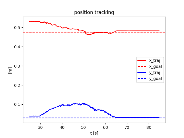
Stabilizing contact-rich plans
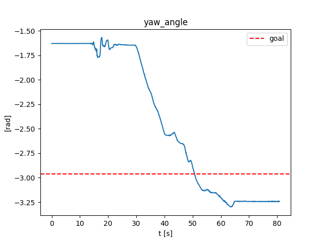
Open-loop hardware
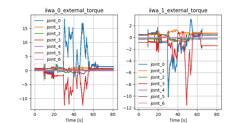
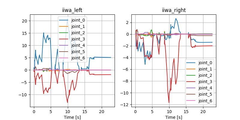
Open-loop Drake
Quasi-static dynamical systems: what it was.
\( x_{+} = f(x, u)\)
- \(x \coloneqq q \coloneqq [q^\mathrm{u}, q^\mathrm{a}]\): system configuration.
- \(q^\mathrm{a}\): actuated, imepdance-controlled robots
- \(q^\mathrm{u}\): un-actuated objects.
- \( u \): robot velocities.
\begin{cases}
\end{cases}
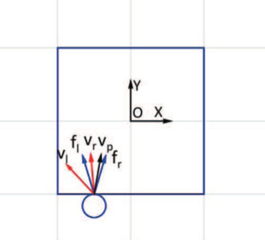
\(\mathrm{v}_p\): applied velocities by the manipulator end effector at the contact point. [1]
[3]
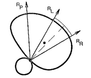
\(R_P\): "the ray of pushing". [2]
This is a good model for planar pushing:
- Contact force cannot be uniquely determined from \(u\) when there is contact.
- As a result, \(q_+\) cannot be determined from \(u\).
- Defining \(u\) as velocity leads to ill-posed dynamical systems (invalid Bond Graphs).
But what about grasping?
- Zhou, Jiaji, et al. "A convex polynomial model for planar sliding mechanics: theory, application, and experimental validation." The International Journal of Robotics Research, 2018.
- Mason, Matthew T. "Mechanics and planning of manipulator pushing operations." The International Journal of Robotics Research, 1986.
- Hogan, François Robert, and Alberto Rodriguez. "Feedback control of the pusher-slider system: A story of hybrid and underactuated contact dynamics." Algorithmic Foundations of Robotics XII, 2020.
What does quasi-dynamic mean?
- Quasi-static \(\Longleftrightarrow \Sigma F = 0\)
- Quasi-dynamic:
"Quasi-dynamic analysis is intermediate between quasi-static and dynamic. Suppose that a manipulation task involves occasional brief periods when there is no quasistatic balance. The task is then governed by Newton's laws. But in some instances, these periods are so brief that the accelerations do not integrate to significant velocities. Momentum and kinetic energy are negligible. Restitution in impact is negligible. It is as if a viscous ether is constantly damping all velocities and sucking the kinetic energy out of all moving bodies. We can analyze such a system by assuming it is at rest, calculating the total forces and body accelerations, then moving each body some short distance in the corresponding direction." -- Matt Mason <Dynamics of Robotic Manipulation>
-
But why is it a good idea?
-
Benefits of quasi-static dynamics for planning:
- Smaller state space (\([q, v]\) vs. only \(q\)).
Larger time steps.
Quasi-dynamic is quasi-static with regularization.
-
\mathbf{M}\ddot{q} + \mathbf{C}(q, \dot{q}) \dot{q} = \tau
0 = \tau
Second-order
mass matrix
Quasi-static
Coriolis Force
Torque (contact + actuation)
\mathbf{M}\ddot{q} = \tau
Quasi-dynamic
Before my PhD defense in December 2022...
- Stabilize this with MPC.
- Already done in Drake.
- Potential problems:
- Robustness.
- Shape variation.
- Coefficient of friction.
- etc.
- Robustness.
- Imperfect actuators.
- Poor tracking.
- Hysteresis.
Turning the ball by 30 degrees: open-loop
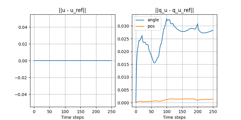
- Simulated in Drake with the same SDF as the quasi-dynamic model used for planning.
Turning the ball by 30 degrees: open-loop with disturbance
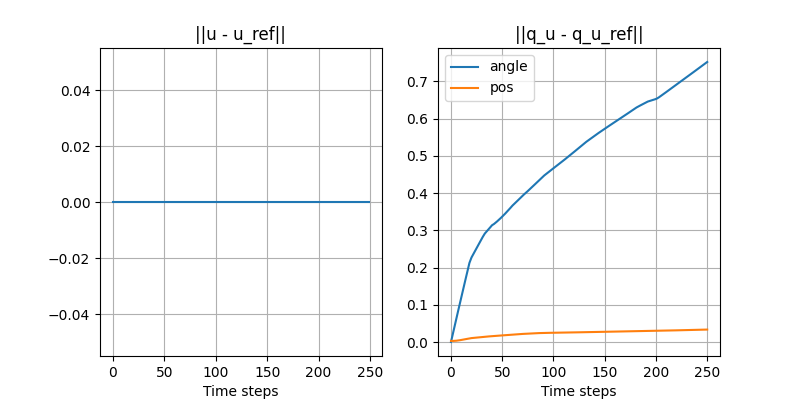
- Initial position of the ball is off by 3mm.
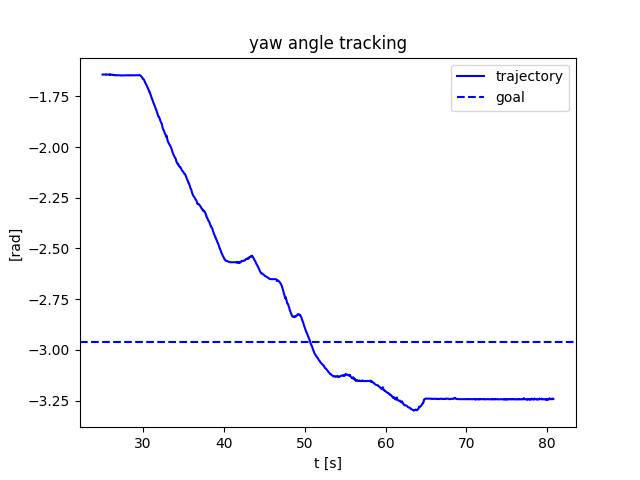
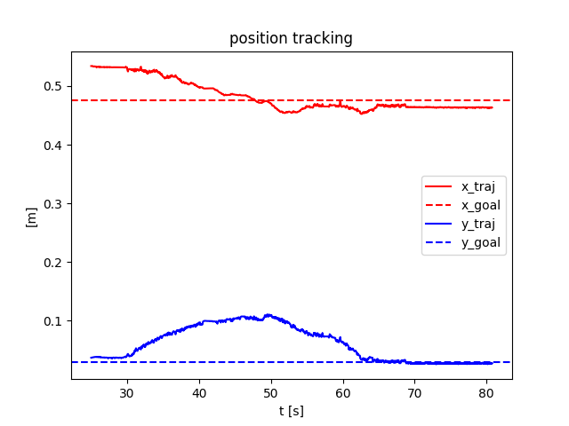
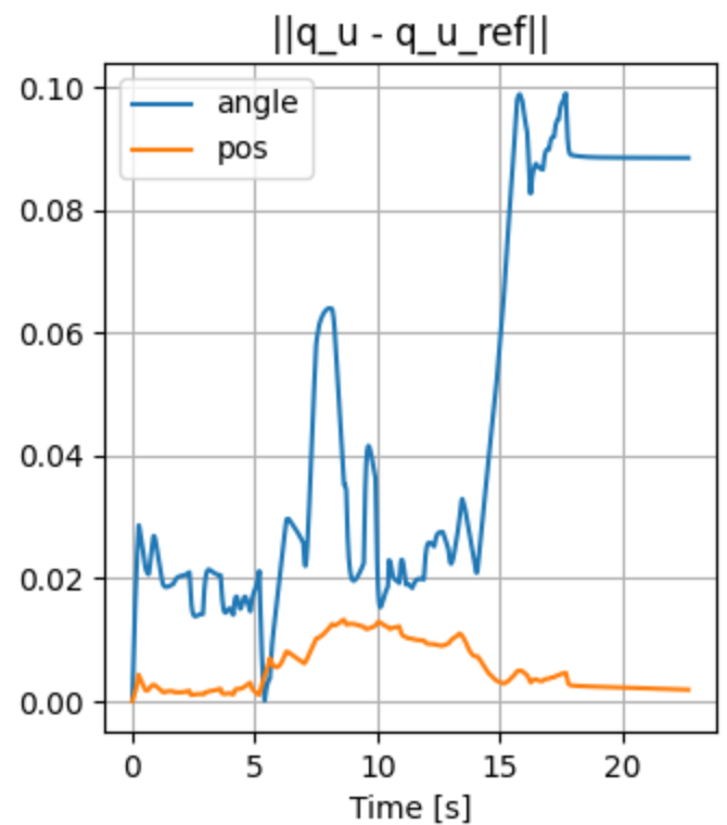
Turning the ball by 30 degrees: closed-loop with disturbance
- Initial position of the ball is off by 3mm.
- Simple controller:
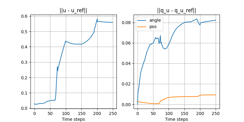
\begin{aligned}
\underset{q^\mathrm{u}_+, u}{\min} &\|q_+^\mathrm{u} - q_+^\mathrm{u, ref}\|_\mathbf{Q} + \|u - u^\mathrm{ref} \|_\mathbf{R}, \text{s.t.}\\
& q^\mathrm{u}_+ = \mathbf{A}_\rho^\mathrm{u} q^\mathrm{u} + \mathbf{B}_\rho^\mathrm{u} u
\end{aligned}
Smooth linearization
talk
By Pang


