AutoGrad
Peter
Intro
Deep leaning
Gradient Based learning
How to Compute Gradient?
1. Symbolic Diff
Use Symbol
like what you do in Calculus class
f (x)= x^3 + x + 1
f'(x) = 3x^2 +1
->
Sympy
2.Numerical Diff
Approximate the derivative
f'(x) = \frac{f(x+h) - f(x)}{h}
Simplest
3. Automatic Diff
Build Computational Graph
Computational Graph
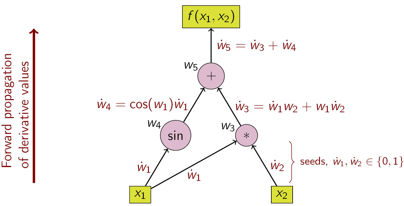
wiki
f (x_1, x_2) = cos(x_1) + x1*x2
Two kinds of Computational Graph
Static v.s. Dynamic
Static
- Theano
- Tensorflow
- Caffe
- Mxnet
Dynamic
- PyTorch
- Mxnet
- Tensorflow Fold
Dynamic
Dynamic
TensorFlow Fold
Pros & Cons
Static pros
- Optimization
- Portable
Static cons
- Hard to debug
- Controll flow
Dynamic
- Easy to debug
- Control flow
- Dynamic structure
Autograd
Compute Gradient in
Plain Python
>>> import autograd.numpy as np  # Thinly-wrapped numpy
>>> from autograd import grad    # The only autograd function you may ever need
>>>
>>> def tanh(x):                 # Define a function
...     y = np.exp(-x)
...     return (1.0 - y) / (1.0 + y)
...
>>> grad_tanh = grad(tanh)       # Obtain its gradient function
>>> grad_tanh(1.0)               # Evaluate the gradient at x = 1.0
0.39322386648296376
>>> (tanh(1.0001) - tanh(0.9999)) / 0.0002  # Compare to finite differences
0.39322386636453377
>>> import matplotlib.pyplot as plt
>>> x = np.linspace(-7, 7, 200) # grad broadcasts across inputs
>>> plt.plot(x, tanh(x),
... x, grad(tanh)(x), # first derivative
... x, grad(grad(tanh))(x), # second derivative
... x, grad(grad(grad(tanh)))(x), # third derivative
... x, grad(grad(grad(grad(tanh))))(x), # fourth derivative
... x, grad(grad(grad(grad(grad(tanh)))))(x), # fifth derivative
... x, grad(grad(grad(grad(grad(grad(tanh))))))(x)) # sixth derivative
>>> plt.show()

Extendable
import autograd.numpy as np
from autograd.core import primitive

@primitive
def logsumexp(x):
    """Numerically stable log(sum(exp(x)))"""
    max_x = np.max(x)
    return max_x + np.log(np.sum(np.exp(x - max_x)))

def logsumexp_vjp(g, ans, vs, gvs, x):
    return np.full(x.shape, g) * np.exp(x - np.full(x.shape, ans))

logsumexp.defvjp(logsumexp_vjp)

from autograd import grad
def example_func(y):
	z = y**2
	lse = logsumexp(z)
	return np.sum(lse)

grad_of_example = grad(example_func)
print "Gradient: ", grad_of_example(np.array([1.5, 6.7, 1e-10])
Support Complex Number!
Multivariable function
import autograd.numpy as np
from autograd import grad

def sigmoid(x):
    return 0.5*(np.tanh(x) + 1)

def logistic_predictions(weights, inputs):
    # Outputs probability of a label being true according to logistic model.
    return sigmoid(np.dot(inputs, weights))

def training_loss(weights):
    # Training loss is the negative log-likelihood of the training labels.
    preds = logistic_predictions(weights, inputs)
    label_probabilities = preds * targets + (1 - preds) * (1 - targets)
    return -np.sum(np.log(label_probabilities))

# Build a toy dataset.
inputs = np.array([[0.52, 1.12,  0.77],
                   [0.88, -1.08, 0.15],
                   [0.52, 0.06, -1.30],
                   [0.74, -2.49, 1.39]])
targets = np.array([True, True, False, True])

# Define a function that returns gradients of training loss using autograd.
training_gradient_fun = grad(training_loss)

# Optimize weights using gradient descent.
weights = np.array([0.0, 0.0, 0.0])
print "Initial loss:", training_loss(weights)
for i in xrange(100):
    weights -= training_gradient_fun(weights) * 0.01

print  "Trained loss:", training_loss(weights)
Q&A
AutoGrad
By Peter Cheng


