Super-efficiency of automatic differentiation for functions defined as a minimum

https://arxiv.org/abs/2002.03722

Pierre Ablin

Joint work with Gabriel Peyré and Thomas Moreau

ICML 2020

10/05/2021

Optimization topic group

Introduction to automatic differentiation

[Baydin et al., 2015, Automatic differentiation in machine learning: a survey]

https://arxiv.org/abs/1502.05767

Automatic differentiation ?

- Method to compute the differential of a function using a computer

Input

def f(x):
  return x ** 2


f(1.)
>>>> 1.

Output

g = grad(f)


g(1.)
>>>> 2.0

Automatic differentiation ?

- Method to compute the differential of a function using a computer

Input

def f(x):
  return np.log(1 + x ** 2) / x


f(1.)
>>>> 0.6931471805599453

Output

g = grad(f)


g(1.)
>>>> 0.3068528194400547

Prototypical case

$f$ defined recursively:

$f_0(x) = x$
$f_{k+1}(x) = 4 f_{k}(x) (1 - f_k(x))$

Input

def f(x, n=4):
  v = x
  for i in range(n):
    v = 4 * v * (1 - v)
  return v


f(0.25)
>>>> 0.75

Output

g = grad(f)


g(0.25)
>>>> -16.0

Automatic differentiation is not...

Numerical differentiation

$$f'(x) \simeq \frac{f(x + h) - f(x)}{h}$$

In higher dimension:

$$ \frac{\partial f} {\partial x_i} (\mathbf{x}) \simeq \frac{f(\mathbf{x} + h \mathbf{e}_i) - f(\mathbf{x})}{h}$$

Drawbacks:

Computing $\nabla f = [\frac{\partial f}{\partial x_1}, \cdots, \frac{\partial f}{\partial x_n}]$ takes $n$ computations
Inexact method
How to choose $h$?

Automatic differentiation is not...

Numerical differentiation

Example:

from scipy.optimize import approx_fprime


approx_fprime(0.25, f, 1e-7)
>>>> -16.00001599

Automatic differentiation is not...

Symbolic differentiation

- Takes as input a function specified as symbolic operations

- Apply the usual rules of differentiation to give the derivative as symbolic operations

Example:

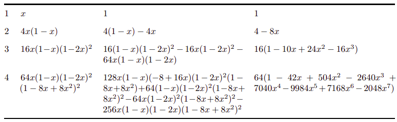
$f_4(x) = 64x(1−x)(1−2x)^2 (1−8x+ 8x^2 )^2$, so:

f'_4(x) = 128x(1 − x)(−8 + 16x)(1 − 2x)^2(1 − 8x+ 8x^2)+ 64(1−x)(1−2x)^2(1−8x+ 8x^2)^2−64x(1 − 2x)^2(1 − 8x+ 8x^2)^2 − 256x(1 − x)(1 −2x)(1 − 8x + 8x^2 )^2

Then, evaluate $f'(x)$

Automatic differentiation is not...

Symbolic differentiation

- Exact

- Expression swell: derivatives can have many more terms than the base function

$f_n$ $f'_n$ $f'_n$ (simplified)

Automatic differentiation:

Apply symbolic differentiation at the elementary operation level and keep intermediate numerical results, in lockstep with the evaluation of the main function.

- Function = graph of elementary operations

- Follow the graph and differentiate each operation using differentiation rules (linearity, chain rule, ...)

def f(x, n=4):
  v = x
  for i in range(n):
    v = 4 * v * (1 - v)
  return v


f(0.25)
>>>> 0.75

def g(x, n=4):
  v, dv = x, 1.
  for i in range(n):
    v, dv = 4 * v * (1 - v), 4 * dv * (1 - v) - 4 * v * dv
  return dv


g(0.25)
>>>> -16.0

Forward automatic differentiation:

Apply symbolic differentiation at the elementary operation level and keep intermediate numerical results, in lockstep with the evaluation of the main function.

- Function = graph of elementary operations

- Follow the graph and differentiate each operation using differentiation rules (linearity, chain rule, ...)

- If $f:\mathbb{R}\to \mathbb{R}^m$: need one pass to compute all derivatives :)

- If $f:\mathbb{R}^n \to \mathbb{R}$: need $n$ passes to compute all derivatives :(

- Bad for ML

Reverse automatic differentiation: Backprop

- Function = graph of elementary operations

- Compute the graph and its elements

- Go through the graph backwards to compute the derivatives

def f(x, n=4):
  v = x
  for i in range(n):
    v = 4 * v * (1 - v)
  return v


f(0.25)
>>>> 0.75

def g(x, n=4):
  v = x
  memory = []
  for i in range(n):
    memory.append(v)
    v = 4 * v * (1 - v)
  dv = 1
  for v in memory[::-1]:
    dv = 4 * dv * (1 - v) - 4 * dv * v
  return dv


g(0.25)
>>>> -16.0

Reverse automatic differentiation: Backprop

- Function = graph of elementary operations

- Compute the graph and its elements

- Go through the graph backwards to compute the derivatives

-Only one passe to compute gradients of functions $\mathbb{R}^n \to \mathbb{R}$ :)

Example on a 2d function

$$f(x, y) = yx^2, \enspace x = y= 1$$

Function

$x =1$

$y = 1$

$v_1 = x^2 = 1$

$v_2 =yv_1 = 1$

$f = v_2 =1$

Forward AD (w.r.t. $x$)

Backprop 

$\frac{dx}{dx} =1$

$\frac{dy}{dx} = 0$

$\frac{dv_1}{dx} =2x \frac{dx}{dx} = 2$

$\frac{dv_2}{dx} =y\frac{dv_1}{dx} +v_1 \frac{dy}{dx} =2$

$\frac{df}{dx} = \frac{dv_2}{dx}=2$

$\frac{df}{dv_2}= 1$

$\frac{df}{dy} = \frac{df}{dv_2 }\frac{dv_2}{dy} = \frac{df}{dv_2 }v_1 = 1$

$\frac{df}{dv_1} =y\frac{df}{ dv_2} = 1$

$\frac{df}{dx} = 2 x \frac{df}{dv_1} = 2$

Automatic differentiation:

- Exact

- Takes about the same time to compute the gradient and the function

- Requires memory: need to store intermediate variables

- Easy to use

- Available in Pytorch, Tensorflow, jax, package autograd with numpy

from autograd import grad

g = grad(f)


g(0.25)
>>>> -16.0

Questions ?

Automatic differentiation for optimization

Example 1: Learning to learn

Ridge regression: minimize $\ell(\beta) = \frac12 \| X \beta - y\|^2 + \frac\lambda 2\|\beta\|^2$

Gradient descent with step $\rho > 0$ for $T$ iterations:

- $\beta_0 = 0$

- $\beta_{t+1} = \beta_t - \rho( X^{\top}(X\beta -y) + \lambda \beta)$

We see it as a function $GD:\rho \to \beta_T$.

What is the best $\rho$ ?

[Gregor, Lecun, 2010, Learning Fast Approximations of Sparse Coding]

Example 1: Learning to learn

Ridge regression: minimize $\ell(\beta) = \frac12 \| X \beta - y\|^2 + \frac\lambda 2\|\beta\|^2$

We want to find $\rho$ that minimizes $\ell(GD(\rho))$

$\to$ use gradient descent!

$$ \rho \leftarrow \rho - 0.01 \nabla_{\rho}\ell(GD(\rho))$$

$\nabla_{\rho}\ell(GD(\rho))$ is computed using automatic differentiation

Example 2: hyperparameter optimization

Ridge regression: minimize $\ell(\beta, \lambda) = \frac12 \| X \beta - y\|^2 + \frac\lambda 2\|\beta\|^2$

- Assume we have a test set $X_{test}, y_{test}$. Minimize test error:

$$\ell'(\beta) = \frac12\|X_{test}\beta - y_{test}\|^2$$

subject to :

$$ \beta = \arg\min \ell(\beta, \lambda)$$

- In this simple case, closed-form solution for $\beta$, but not in general

[Bengio, 1990, Gradient based optimization of hyperparameters]

Example 2: hyperparameter optimization

Ridge regression: minimize $\ell(\beta, \lambda) = \frac12 \| X \beta - y\|^2 + \frac\lambda 2\|\beta\|^2$

$$ \min \ell'(\beta) = \frac12\|X_{test}\beta - y_{test}\|^2 \enspace \text{s.t.} \enspace \beta = \arg\min \ell(\beta, \lambda)$$

- Define the output of gradient descent $GD: \lambda \to \beta$:

$$GD(\lambda) \simeq \argmin_{\beta} \ell(\beta, \lambda)$$

- Optimize $\ell'(GD(\lambda))$ with gradient descent, using autodiff to compute the gradient

Better scaling with # of hyperparameters than grid-search

Questions ?

Super efficiency of autodiff for functions defined as a minimum

https://arxiv.org/abs/2002.03722

Setting:

\ell(x) = \min_z \mathcal{L}(z, x)

- Minimization not in closed-form : sequence $z_t(x)$ produced by e.g. gradient descent such that $\mathcal{L}( z_t(x), x) \to \ell(x)$

- How can we estimate $ \nabla \ell(x)$ using $z_t(x)$?

- Use $\nabla \ell(x)$ e.g. to minimize / maximize $\ell$

The analytic estimator

\ell(x) = \min_z \mathcal{L}(z, x)

- Assume $\mathcal{L}$ is differentiable and there is $z^*(x)$ such that $\ell(x)=\mathcal{L}(z^*(x), x)$

$$\nabla_x\ell(x) = J^*\underbrace{\nabla_z \mathcal{L}(z^*(x), x)}_{=0 } + \nabla_x \mathcal{L}(z^*(x), x)$$

$J^*= \frac{\partial z^*}{\partial x}$ is the Jacobian of $z^*$

$$\nabla_x\ell(x) = \nabla_x \mathcal{L}(z^*(x), x)$$

The analytic estimator

\ell(x) = \mathcal{L}(z^*(x), x)

- Given a sequence $z_t(x)$ approaching $z^*(x)$, the analytic estimator is:

$$\nabla_x\ell(x) = \nabla_x \mathcal{L}(z^*(x), x)$$

g^1_t(x) = \nabla_x \mathcal{L}(z_t(x), x)

If $\nabla_x \mathcal{L} $ is $L-$Lipschitz:

$$ |g^1_t (x) - \nabla_x \ell(x)| \leq L |z_t(x) - z^*(x)|$$

$g^1$ converges at the same speed as $z_t$

The autodiff estimator

\ell(x) = \mathcal{L}(z^*(x), x)

- Given a sequence $z_t(x)$ approaching $z^*(x)$, the autodiff estimator is:

g^2_t(x) = \frac{\partial}{\partial x}\left[ \mathcal{L}(z_t(x), x)\right]

Derivative with respect to $z_t(x)$ as well:

$$g^2_t(x) = \nabla_x\mathcal{L}(z_t, x) + J_t\nabla_z\mathcal{L}(z_t, x)$$

$J_t = \frac{\partial z_t}{\partial x}$ is the Jacobian of $z_t$

-$g^2_t$ can be computed at ~ the same cost as $z_t$using autodiff

The autodiff estimator

Look at second order expansions:

$$\nabla_x\mathcal{L}(z_t, x) = \nabla_x \ell(x) + \nabla_{xz}\mathcal{L}(z^*, x)(z_t -z^*) + R_{xz}$$

$$\nabla_z\mathcal{L}(z_t, x) =\nabla_{zz}\mathcal{L}(z^*, x) (z_t - z^*) + R_{zz}$$

Rests are $R_{xz}, R_{zz} = O(|z_t - z^*|^2)$.

Jacobian error:

$$R(J) = J \nabla_{zz}\mathcal{L}(z^*, x) + \nabla_{xz}\mathcal{L}(z^*, x)$$

$$g^2_t(x) = \nabla_x\mathcal{L}(z_t, x) + J_t\nabla_z\mathcal{L}(z_t, x)$$

g^2_t - \nabla_x \ell(x) = R(J_t)(z_t - z^*) + R_{xz} + J_t R_{zz}

The autodiff estimator

g^2_t - \nabla_x \ell(x) = \underbrace{R(J_t)(z_t - z^*)}_{?} + \underbrace{R_{xz} + J_t R_{zz}}_{O(|z_t - z^*|^2)}

Implicit functions theorem:

$$R(J^*) = J^* \nabla_{zz}\mathcal{L}(z^*, x) + \nabla_{xz}\mathcal{L}(z^*, x) = 0$$

So if $J_t \to J^*$ (more later), $R(J_t) \to 0$ and:

g^2_t = \nabla_x \ell(x) + o(|z_t - z^*|)

$g^2$ converges faster than $z_t$

The implicit estimator

Recall:

$$\nabla_x\ell(x) = J^*\nabla_z \mathcal{L}(z^*(x), x) + \nabla_x \mathcal{L}(z^*(x), x)$$

Implicit function theorem:

$$J^* = - \nabla_{xz}\mathcal{L}(z^*, x) \left[\nabla_{zz}\mathcal{L}(z^*, x)\right]^{-1} = \mathcal{J}(z^*, x)$$

Implicit estimator:

$$g^3_t = \mathcal{J}(z_t, x) \nabla_z \mathcal{L}(z_t, x) + \nabla_x \mathcal{L}(z_t, x)$$

The implicit estimator

$$g^3_t = \mathcal{J}(z_t, x) \nabla_z \mathcal{L}(z_t, x) + \nabla_x \mathcal{L}(z_t, x)$$

Just like $g^2$, we have:

Hence if $R(\mathcal{J}(z_t, x)) = O(|z_t - z^*|)$:

$$ g^3_t = \nabla_x \ell(x) + O(|z_t - z^*|^2)$$

g^3_t - \nabla_x \ell(x) = R(\mathcal{J}(z_t, x))(z_t - z^*) + R_{xz} + R(\mathcal{J}(z_t, x)) R_{zz}

$g^3$ converges twice as fast as $z_t$

So far...

$$g^1 - \nabla_x \ell \simeq \enspace z_t - z^*\enspace$$

$$g^2 - \nabla_x \ell <\enspace z_t - z^*\enspace$$

$$g^3 - \nabla_x \ell \simeq (z_t - z^*)^2$$

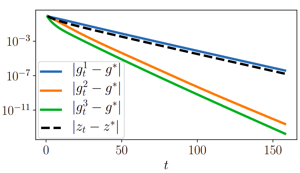
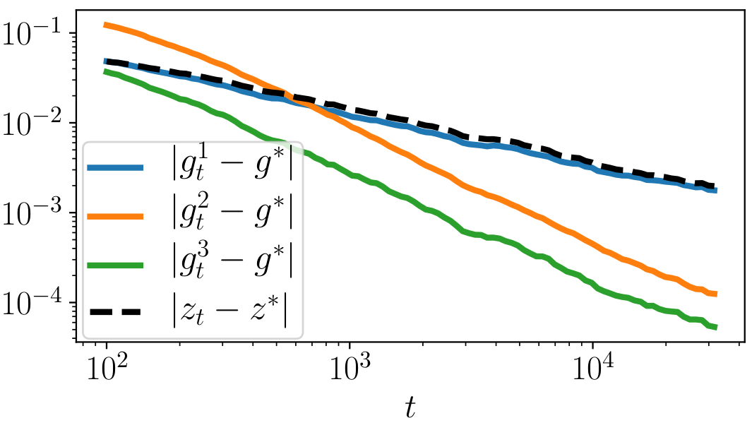
Example on a logistic loss:

$$\mathcal{L}(z, x) = \sum_{i=1}^n \log(1 + \exp(- x_i [Dz]_i)) + \lambda \|z\|^2$$

$z_t$ obtained with gradient descent:

Tighter analysis of the autodiff estimator

Recall:

$$g^2 - \nabla_x \ell = R(J_t) (z_t - z^*) + O(|z_t - z^*|^2)$$

We want to analyse $R(J_t)$.

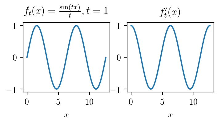
Assume $z_t(x) \to z^*(x)$, do we have

$$J_t = \frac{\partial z_t(x)}{\partial x} \to J^* = \frac{\partial z^*(x)}{\partial x}?$$

In general, no :(

$$z_t(x) = \frac1t\sin(tx) \rightarrow 0$$

$$J_t = \cos(tx) \nrightarrow 0$$

Tighter analysis of the autodiff estimator

Assume $\mathcal{L}$ is $\mu$-strongly convex and $L$-smooth w.r.t. $z$, and that $z_t$ is obtained by gradient descent:

$$z_{t+1}(x) = z_t(x) - \rho \nabla_z\mathcal{L}(z_t(x), x)$$

Then,

$$|z_t - z^*| = O(\kappa^t)$$

$$\|J_t - J^*\| = O(t \kappa^t), \enspace \kappa = 1 - \rho \mu$$

We obtain $z^t$ using optimization methods $\to$ no such problem.

Theorem:

$J_t$ converges slightly slower than $z_t$

Bounds in the strongly convex setting

Assume $\mathcal{L}$ is $\mu$-strongly convex and $L$-smooth w.r.t. $z$, and that $z_t$ is obtained by gradient descent:

$$z_{t+1}(x) = z_t(x) - \rho \nabla_z\mathcal{L}(z_t(x), x)$$

Then,

$$g^1 - \nabla_x\ell(x) = \enspace O(\kappa^{t})$$

$$g^2 - \nabla_x\ell(x) = O(t\kappa^{2t})$$

$$g^3 - \nabla_x\ell(x) = \enspace O(\kappa^{2t})$$

Beyond linear convergence

For SGD / a class of non-strongly convex functions (p-Lojasiewicz), we get:

$$g^1 - \nabla_x\ell(x) = O(z_t - z^*)\enspace \enspace$$

$$g^2 - \nabla_x\ell(x) = O((z_t-z^*)^2)$$

$$g^3 - \nabla_x\ell(x) = O((z_t-z^*)^2)$$

SGD example:

In practice:

In the linear convergence case:

$$g^1 - \nabla_x\ell(x) = \enspace O(\kappa^{t})$$

$$g^2 - \nabla_x\ell(x) = O(t\kappa^{2t})$$

$$g^3 - \nabla_x\ell(x) = \enspace O(\kappa^{2t})$$

But...

-Computing $g^2$ is about twice as costly as $g^1$ $\to$ pointless to use $g^2$

$$g^2_{t} \simeq g^1_{2t}$$

-Computing $g^3$ involves matrix inversion / big operators

In practice:

In the sub-linear convergence case:

$$g^1 - \nabla_x\ell(x) = O(1 / t)\enspace$$

$$g^2 -\nabla_x\ell(x) = O(1 / t^2)$$

$$g^3 - \nabla_x\ell(x) = O(1 / t^2)$$

-Much better to use $g^2$ than $g^1$

Thanks for you attention !

autodiff

By Pierre Ablin

Super-efficiency of automatic differentiation for functions defined as a minimum

Introduction to automatic differentiation

Automatic differentiation ?

Automatic differentiation ?

Prototypical case

Automatic differentiation is not...

Automatic differentiation is not...

Automatic differentiation is not...

Automatic differentiation is not...

Automatic differentiation:

Forward automatic differentiation:

Reverse automatic differentiation: Backprop

Reverse automatic differentiation: Backprop

Example on a 2d function

Automatic differentiation:

Questions ?

Automatic differentiation for optimization

Example 1: Learning to learn

Example 1: Learning to learn

Example 2: hyperparameter optimization

Example 2: hyperparameter optimization

Questions ?

Super efficiency of autodiff for functions defined as a minimum

Setting:

The analytic estimator

The analytic estimator

The autodiff estimator

The autodiff estimator

The autodiff estimator

The implicit estimator

The implicit estimator

So far...

Tighter analysis of the autodiff estimator

Tighter analysis of the autodiff estimator

Bounds in the strongly convex setting

Beyond linear convergence

In practice:

In practice:

Thanks for you attention !

autodiff

More from Pierre Ablin