The LASSO:
least absolute shrinkage and selection operator
Pierre Ablin
12/03/2019
Parietal Tutorial
Overview
- Linear regression
- The Lasso model
- Non-smooth optimization: proximal operators
Supervised learning
y \in \mathbb{R}, \enspace \mathbf{x} \in \mathbb{R}^P, \enspace \varepsilon = \mathcal{N}(0, \sigma^2), \enspace f: \mathbb{R}^P \rightarrow \mathbb{R}
y = f(\mathbf{x}) + \varepsilon
GOAL: Learn \( f \) from some realizations of \( (\mathbf{x}, y) \)
Linear regression
y = f(\mathbf{x}) + \varepsilon
GOAL: Learn \( f \) from some realizations of \( (\mathbf{x}, y) \)
Assumption:
\(f\) is linear
f(\mathbf{x}) = \beta_1x_1 + \beta_2 x_2 + \cdots + \beta_P x_P = \mathbf{x}^{\top} \mathbf{\beta}
GOAL: Learn \( \beta \) from some realizations of \( (\mathbf{x}, y) \)
Maximum likelihood?
y = \mathbf{x}^{\top} \mathbf{\beta} + \varepsilon
For one sample, if we observe \( \mathbf{x}_{\text{obs}}\) and \( y_{\text{obs}} \) , we have:
p(y = y_{\text{obs}} | \mathbf{x} = \mathbf{x}_{\text{obs}}) = p( \mathbf{x}_{\text{obs}}^{\top} \mathbf{\beta} + \varepsilon = y_{\text{obs}}| \mathbf{x} = \mathbf{x}_{\text{obs}})
i.e. :
p(y = y_{\text{obs}} | \mathbf{x} = \mathbf{x}_{\text{obs}}) = p(\varepsilon = y_{\text{obs}} - \mathbf{x}_{\text{obs}}^{\top} \mathbf{\beta})
\\
= \frac{1}{\sqrt{2 \pi \sigma^2}} \exp{(- \frac{( y_{\text{obs}} - \mathbf{x}_{\text{obs}}^{\top} \mathbf{\beta})^2}{2\sigma^2})}
Maximum likelihood?
For one sample, if we observe \( \mathbf{x}_{\text{obs}}\) and \( y_{\text{obs}} \) , we have:
p(y = y_{\text{obs}} | \mathbf{x} = \mathbf{x}_{\text{obs}}) = \frac{1}{\sqrt{2 \pi \sigma^2}} \exp{(- \frac{( y_{\text{obs}} - \mathbf{x}_{\text{obs}}^{\top} \mathbf{\beta})^2}{2\sigma^2})}
If we observe a whole dataset of \(N\) i.i.d. samples$$ (\mathbf{x}_1,y_1), \cdots, (\mathbf{x}_N, y_N) \enspace, $$
the likelihood of this observation is:
\mathcal{L}(\beta) = p(y_1 = y_1, \cdots, y_N = y_N | \mathbf{x}_1 = \mathbf{x}_1, \cdots, \mathbf{x}_N=\mathbf{x}_N)
\\
= p(y_1 = y_1| \mathbf{x}_1 = \mathbf{x}_1) \times \cdots \times p(y_N = y_N| \mathbf{x}_N = \mathbf{x}_N)
\\
maximum likelihood estimator:
\beta_{\text{MLE}} = \arg\max \mathcal{L}(\beta) = \arg\min \sum_{n=1}^N \frac12 (y_n - \mathbf{x}_n^{\top} \beta)^2
Matrix interlude
Define the \(\ell_2\) norm of a vector:
$$|| \mathbf{v}|| = \sqrt{\sum_{n=1}^N v_n^2}$$
And note in condensed matrix form:
$$ \mathbf{y} = [y_1,\cdots, y_N]^{\top} \in \mathbb{R}^N$$
X = [\mathbf{x}_1,\cdots,\mathbf{x}_N]^{\top}\in\mathbb{R}^{N \times P}
Then,
\sum_{n=1}^N (y_n - \mathbf{x}_n^{\top} \beta)^2 = ||\mathbf{y} - X \beta||^2
M.L.E.
\beta_{\text{MLE}} = \arg\min \frac12 ||\mathbf{y} - X \beta||^2
Pros:
- Consistant: as \( N \rightarrow \infty \), \(\beta_{\text{MLE}} \rightarrow \beta^* \)
- Comes from a clear statistical framework
- Can behave badly when the model is mispecified (e.g. \(f\) is not really linear)
- Lots of variance in \(\beta_{\text{MLE}}\) when \(N\) is not big enough
- Ill posed problem when \(N < P\) !
Cons:
What do we do when n < p?
Bet on sparsity / Ockham's razor: only a few coefficients in \( \beta \) play a role
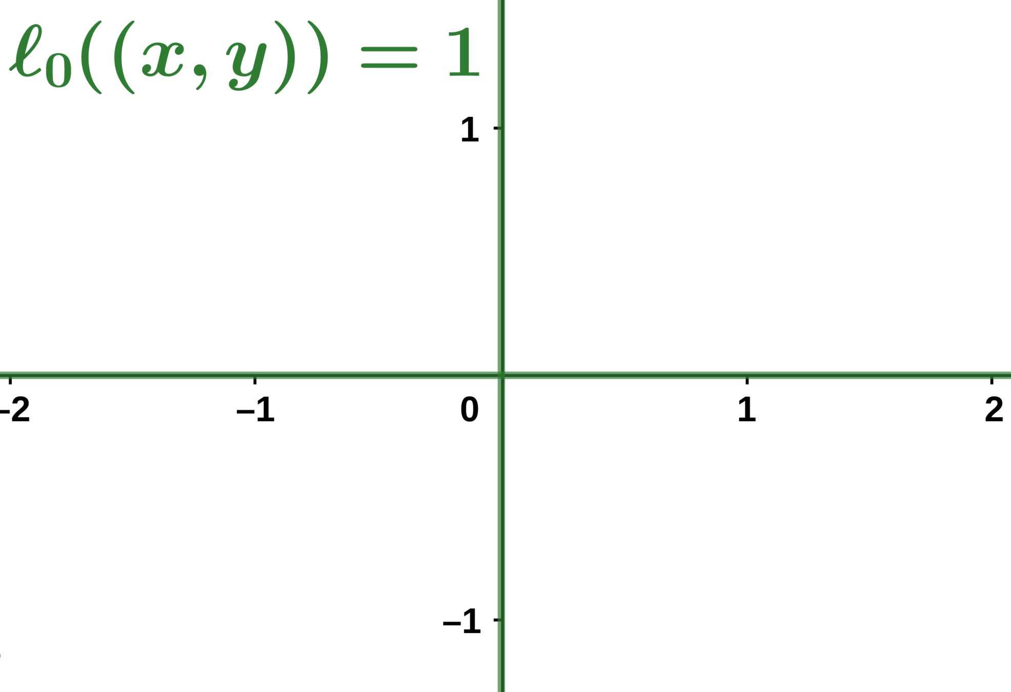
The \( \ell_0 \) Norm:
\ell_0(\beta) = \text{Number of non-zero coefficients in }\beta
Example:
(1.1, 2.5, -6.3, 4.1) \rightarrow 4
\\
(1.1, 0, 0, 4.1) \rightarrow 2
\\
(0, 0, 0, 0) \rightarrow 0
Subset selection/matching pursuit
Idea: select only a few active coefficients with the \( \ell_0 \) norm.
\beta_{\text{subset}} = \arg\min \frac12 || \mathbf{y} - X\beta ||^2 \enspace \text{subject to} \enspace \ell_0(\beta) \leq t
Where \( t\) is an integer controlling the sparsity of the solution.
- Non-convexity
- Instability: adding a sample may completely change \( \beta \) and its support.
- NP-Hard (loooong to solve)
Problems:
The Lasso
Idea: relax the \(\ell_0\) norm to obtain a convex problem
\beta_{\text{lasso}} = \arg\min \frac12 || \mathbf{y} - X\beta ||^2 \enspace \text{subject to} \enspace \ell_1(\beta) \leq t
Where \( t\) is a level controlling the sparsity of the solution.
See notebook
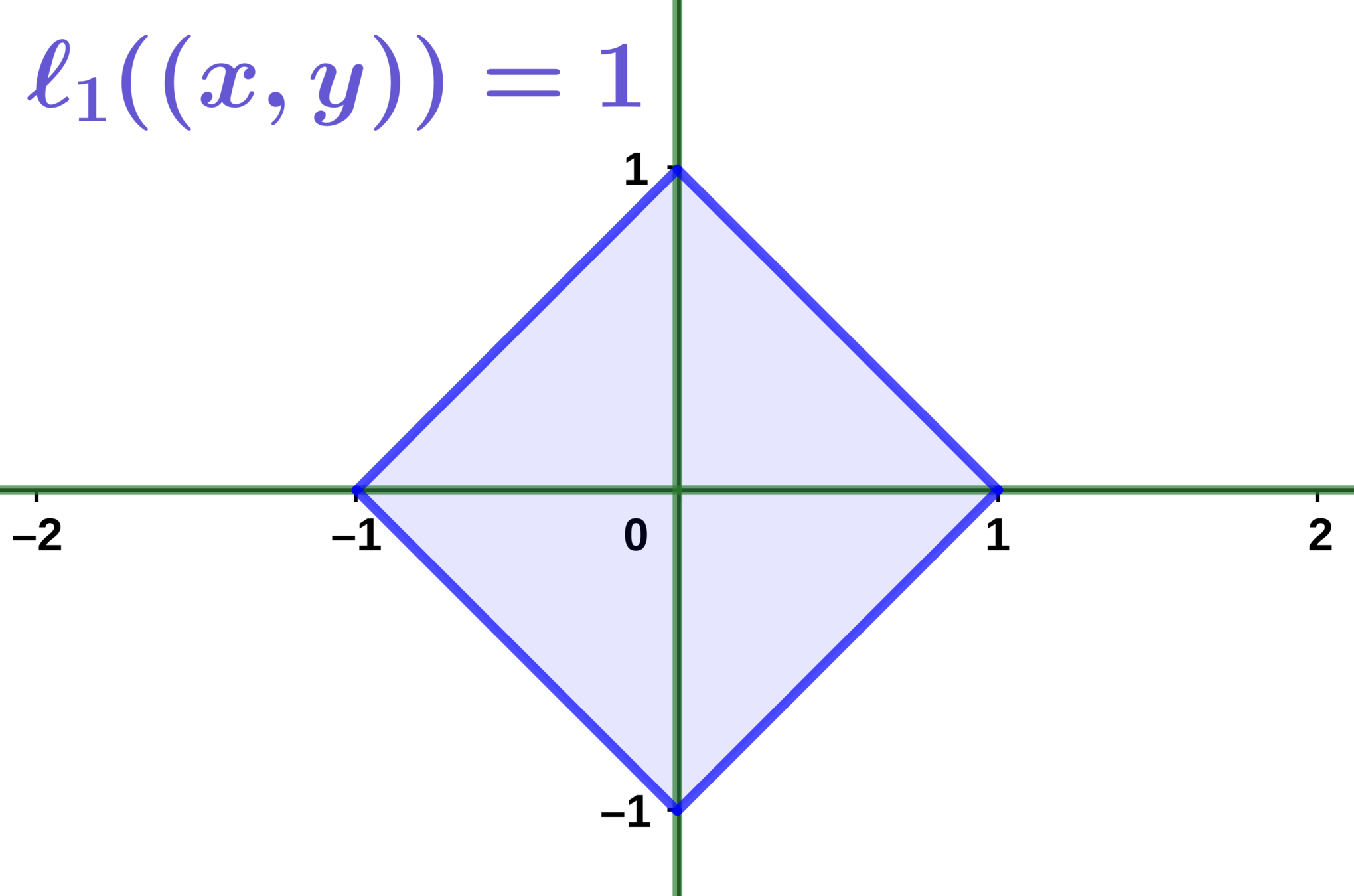
\ell_1(\beta) = |\beta |_1 = |\beta_1| + \cdots + |\beta_P|
The Lasso: Lagrange formulation
\beta_{\text{lasso}} = \arg\min \frac12 || \mathbf{y} - X\beta ||^2 + \lambda |\beta|_1
Where \( \lambda \) is a level controlling the amount of sparsity.
- Relationship between \(\lambda\) and \(t\) depends on the data
- It promotes sparsity: there is a threshold \(\lambda_{\text{max}}\) such that \( \lambda >\) \(\lambda_{\text{max}}\) implies \(\beta_{\text{lasso}} = 0 \)
Derivation
\(\beta = 0\) is a solution to the lasso if:
0 \in \partial_{\beta=0}(\frac12 ||y - X \beta||^2 + \lambda |\beta|_1)
Where \(\partial \) is the subgradient.
\partial(\frac12 || y - X\beta||^2) = \{X^{\top}X\beta - X^{\top} y\}
\partial_{\beta=0}(\lambda|\beta|_1) = [-\lambda, \lambda]^P
So the condition writes:
\forall p, \enspace (X^{\top}y)_p \in [-\lambda , \lambda]
\lambda_{\text{max}} = |X^{\top}y|_{\infty}
Lasso is useful because...
- It performs at the same time model selection and estimation : it tells you which coefficients in \(\mathbf{x}\) are important.
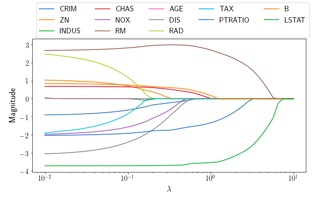
Boston dataset:
Lasso is useful because...
- Leveraging sparsity enables fast solvers
If \(p = 1000 \) and \(n = 1000 \), computing \(X\beta\) takes \(\sim n \times p = 10^6 \) operations
Intuition:
But if we know that there are only \(10 \) non-zero coefficients in \(\beta\), it takes only \(\sim 10^4\) operations
The same reasoning applies to most quantities useful to estimate the model
Lasso estimation
how do we fit the model?
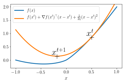
Gradient descent 101
Minimize \( f(\mathbf{x})\) where \(f\) is differentiable.
Iterate \(\mathbf{x}^{t+1} = \mathbf{x}^t - \eta \nabla f(\mathbf{x}^t) \)
Equivalent to minimizing a quadratic surrogate:
\mathbf{x}^{t+1} = \arg\min_{\mathbf{x}} f(\mathbf{x}^t) + \nabla f(\mathbf{x}^t)^{\top}(\mathbf{x} - \mathbf{x}^t) + \frac{1}{2\eta} ||\mathbf{x} - \mathbf{x}^t||_2^2
The simplest lasso:
\(P=1, N = 1, X = 1:\) can we minimize \(\frac12 (y - \beta)^2 + \lambda |\beta|\) ?
Yes: proximity operator
\text{prox}_{|\cdot |}(y, \lambda) = \arg\min_{\beta} \frac12(y-\beta)^2 + \lambda |\beta|
Soft-thresholding:
\text{prox}_{|\cdot |}(y, \lambda) =
- \(0\) if \(|y|\leq \lambda\)
- \(y- \lambda\) if \(y>\lambda\)
- \(y + \lambda\) if \(y < -\lambda\)
Soft thresholding
\text{st}(y, \lambda) =
- \(0\) if \(|y|\leq \lambda\)
- \(y- \lambda\) if \(y>\lambda\)
- \(y + \lambda\) if \(y < -\lambda\)
Separability:
\text{prox}_{|\cdot |_1}(\mathbf{z}, \lambda) = \arg\min_{\beta}\frac12 ||\mathbf{z} - \beta ||^2 + \lambda |\beta|_1 =(\text{st}(z_1, \lambda), \cdots, \text{st}(z_P, \lambda))
ISTA: Iterative soft threshdolding algorithm
\beta_{\text{lasso}} = \arg\min \frac12 || \mathbf{y} - X\beta ||^2 + \lambda |\beta|_1
Gradient of the smooth term:
\nabla_{\beta}(\frac12||\mathbf{y} - X \beta ||^2) = X^{\top}( X \beta - \mathbf{y})
\beta^{t+1} = \text{prox}_{|\cdot|_1}(\beta^{t} - \eta X^{\top}(X\beta^{t} - \mathbf{y}), \lambda\eta)
ISTA:
Comes from:
\mathbf{\beta}^{t+1} = \arg\min_{\beta} f(\mathbf{\beta}^t) + \nabla f(\beta^t)^{\top}(\beta - \beta^t) + \frac{1}{2\eta} ||\beta - \beta^t||_2^2 + \lambda |\beta|_1
ISTA: Iterative soft threshdolding algorithm
\beta^{t+1} = \text{prox}_{|\cdot|_1}(\beta^{t} - \eta X^{\top}(X\beta^{t} - \mathbf{y}), \lambda\eta)
- Some coefficients are \(0\) because of the prox
- One iteration takes \(O(\min(N, P) \times P)\)
Can be problematic for large \(P\) !
COORDInate descent
\beta^{t+1}_j = \text{prox}_{|\cdot|_1}(\beta^{t}_j - \eta X[j, :]^{\top}(X\beta^{t} - \mathbf{y}), \lambda\eta)
Idea : update only one coefficient of \( \beta \) at each iteration.
- If we know the residual \( \mathbf{r} =X\beta^{t} - \mathbf{y}\), each update is \(O(n) \) :)
Residual update:
After updating the coordinate \(j\):
\mathbf{r} \leftarrow \mathbf{r} + (\beta^{\text{new}}_j - \beta^{\text{old}}_j)X[j, :]
\( \beta^{t+1}_i = \beta^{t}_i \) for \( i \enspace \ne j \)
Thanks!
The LASSO
By Pierre Ablin


