


russtedrake PRO
Roboticist at MIT and TRI
Russ Tedrake
Grasp Lab Seminar
October 29, 2021
Slides available live at https://slides.com/d/absz0Qc/live
or later at https://slides.com/russtedrake/2021-grasp
Tobia Marcucci, Jack Umenberger, Pablo Parrilo, Russ Tedrake. Shortest Paths in Graphs of Convex Sets. (Under review)
Available at: https://arxiv.org/abs/2101.11565
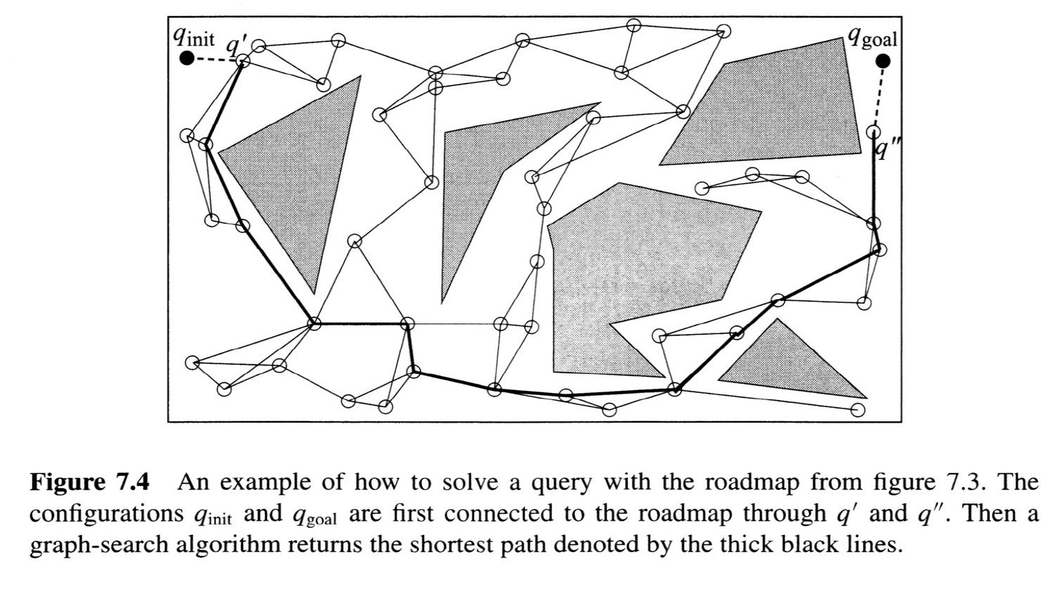
The Probabilistic Roadmap (PRM)
from Choset, Howie M., et al. Principles of robot motion: theory, algorithms, and implementation. MIT press, 2005.
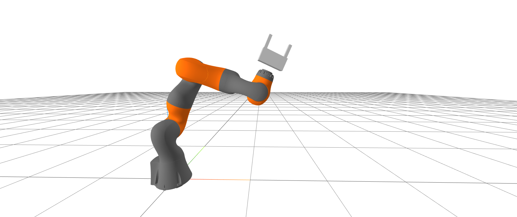
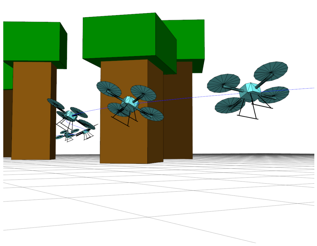
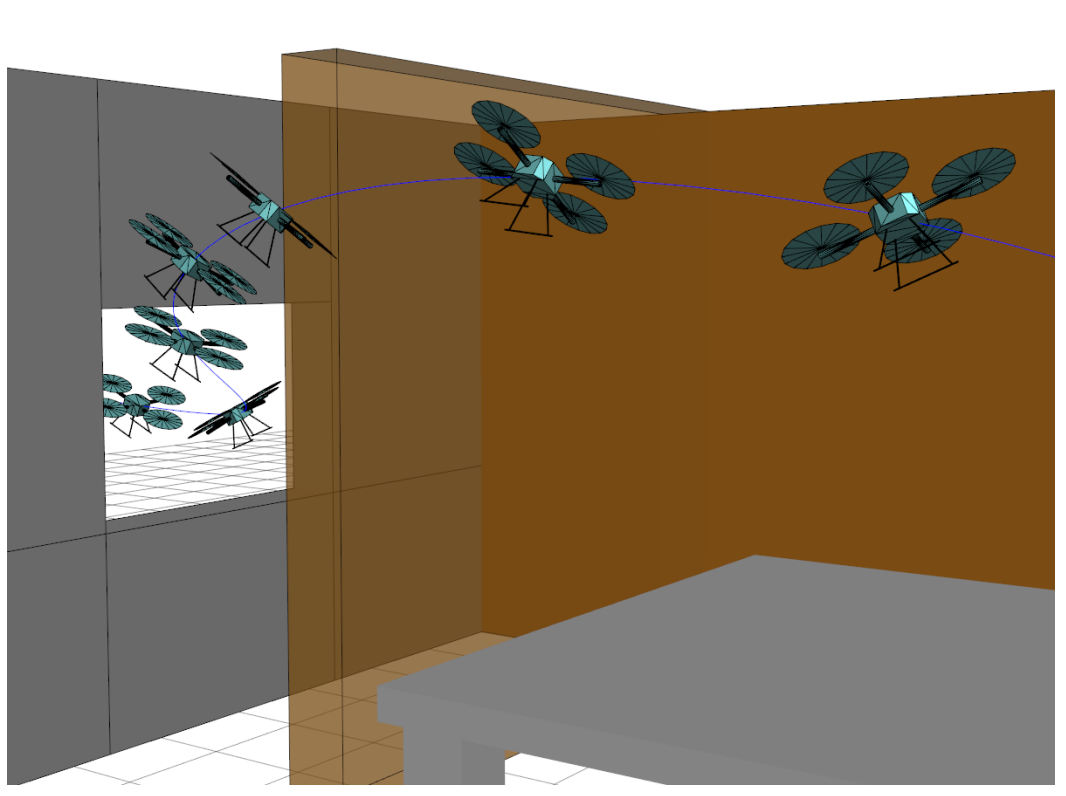
Global optimization-based planning for manipulators with dynamic constraints
image credit: James Kuffner
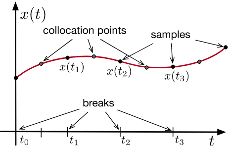
Approximate
Trajectory optimization
Sample-based planning
AI-style logical planning
Combinatorial optimization
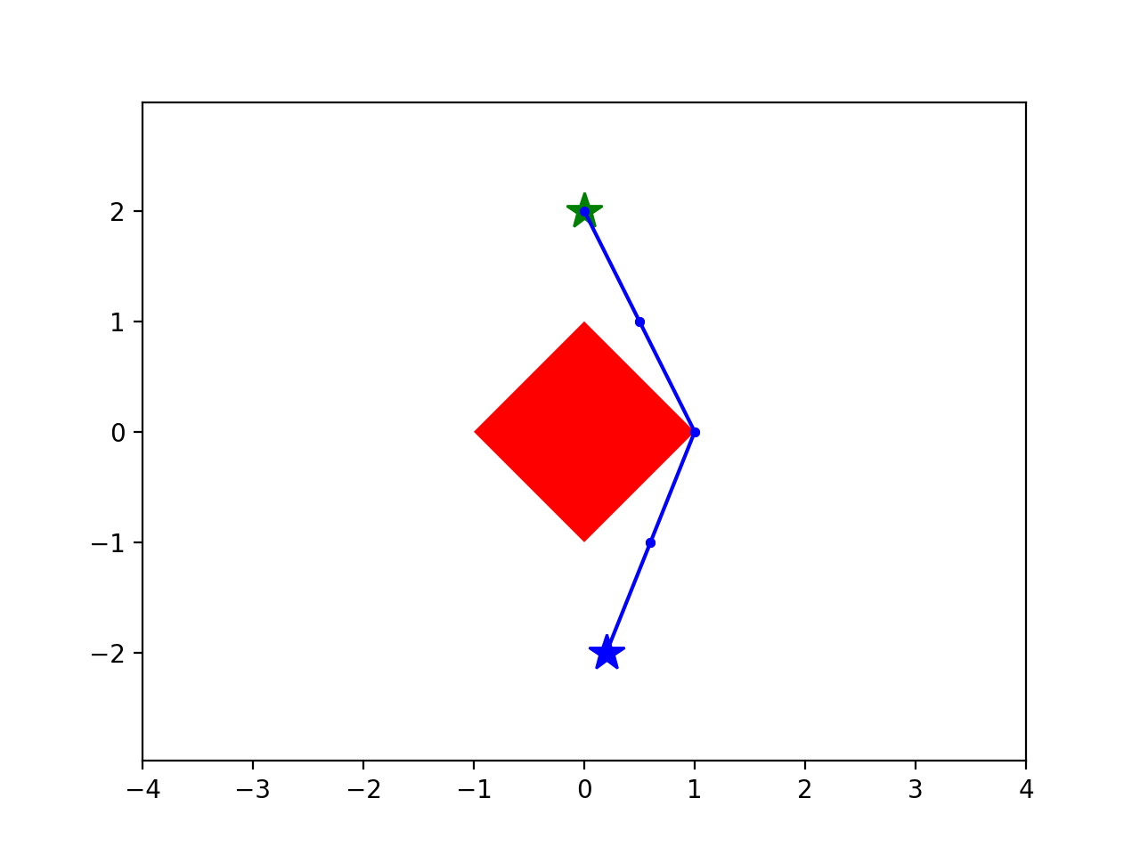
start
goal
Step 1:
Big-M formulation
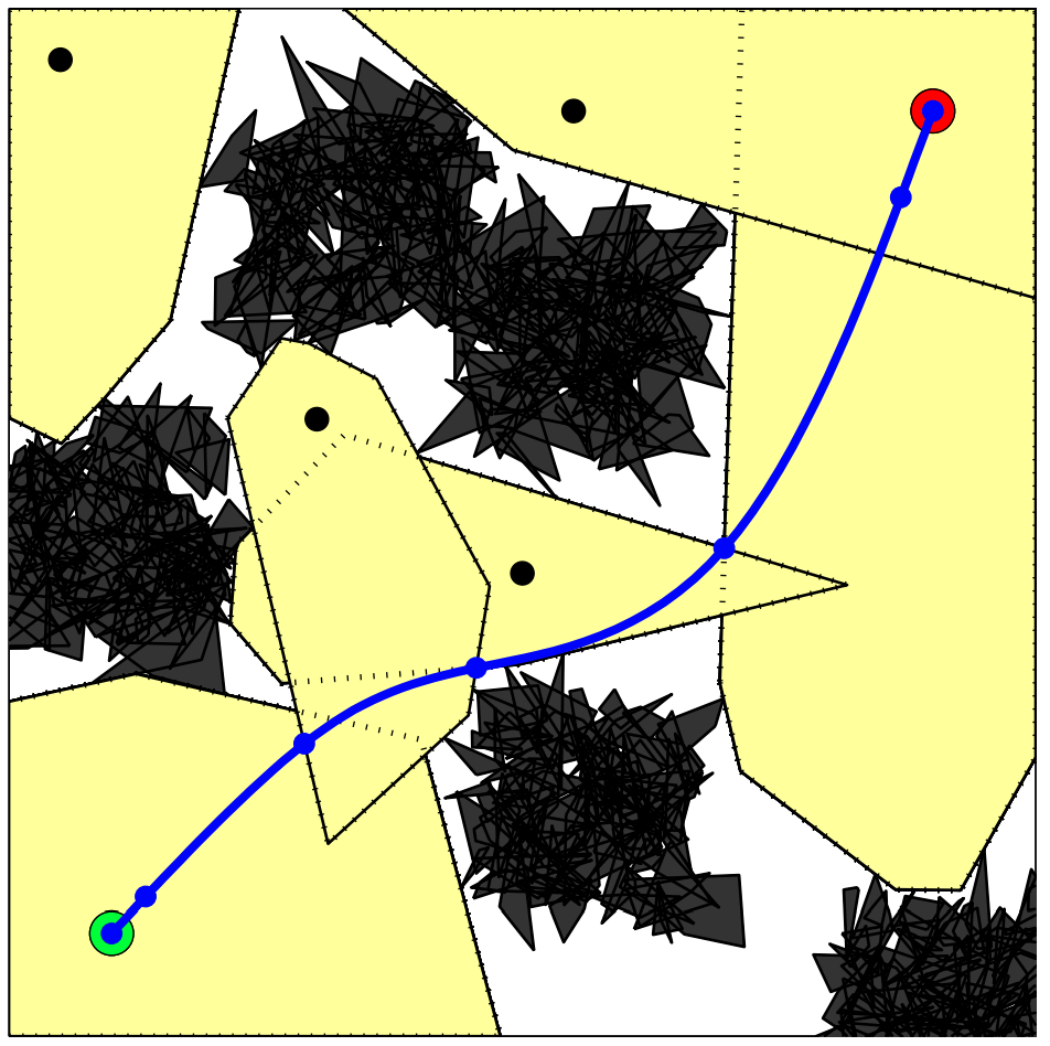
IRIS (Fast approximate convex segmentation)
start
goal
Step 2:
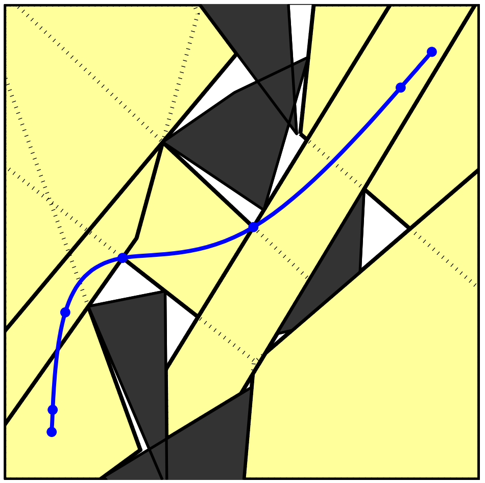
Convex hull formulation
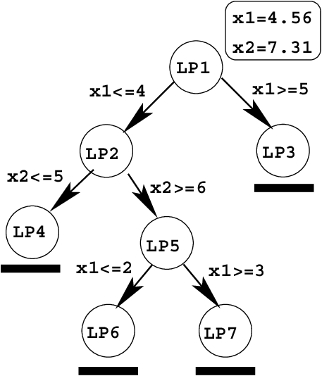
"We know that the LP formulation of the shortest path problem is tight. Why exactly are your relaxations loose?"
\(\varphi_{ij} = 1\) if the edge \((i,j)\) in shortest path, otherwise \(\varphi_{ij} = 0.\)
\(c_{ij} \) is the (constant) length of edge \((i,j).\)
"flow constraints"
binary relaxation
path length
Classic shortest path LP
now w/ Convex Sets
start
goal
Step 3:
New formulation
Note: Path length is no longer predetermined
is the convex relaxation. (it's tight!)
| Previous best formulations | New formulation | |
|---|---|---|
| Lower Bound (from convex relaxation) |
7% of MICP | 80% of MICP |
Going forward...
work w/ Andres Valenzuela
work w/ Soonho Kong
work w/ Mark Petersen
Give it a try:
pip install drake
sudo apt install drakeTrajectory optimization
Sample-based planning
AI-style logical planning
Combinatorial optimization
http://manipulation.mit.edu
By russtedrake
Talk at UIUC, January 19, 2021


