An Invitation to Reinforcement Learning

To fix ideas: Formulation of a DTMC-SIS model 

Nonlinear control: HJB and DP

Given 

\frac{dx}{dt} = f(x(t))

Goal:

Desing

to follow

 s. t. optimize cost    

\text{action } a_t\in \mathcal{A},
\text{state } x_t
\frac{dx_{t}}{dt} =f(x_{t} ,a_{t})

Agent

a_t\in \mathcal{A}
x_t
J(x_t, a_t, 0, T) = Q(x_T, T) + \int_0^T \mathcal{L}(x_{\tau}, a_{\tau}) d_{\tau}
J(x_t, a_t, 0, T) .

Nonlinear control: HJB and DP

V(x_0, 0, T):= \min_{a_t \in \mathcal{A}} J(x_t, a_t, 0, T)
V(x_0, 0, T) = V(x_0, 0, t) + V(x_0, t, T)

Bellman Optimality

Optimal Control Problem

\frac{dx_t}{dt} = f(x_t, a_t)
\min_{a_t\in \mathcal{A}} J(x_t, a_t, 0, T) = Q(x_T, T) + \int_0^T \mathcal{L}(x_{\tau}, a_{\tau}) d_{\tau}

s.t.

x_T
x_t
x_0
\frac{\partial V}{\partial t} = \min_{a_t\in \mathcal{A}} \left[ \left( \frac{\partial V}{\partial x} \right)^{\top} f(x,a) + \mathcal{L}(x,a) \right]

Data

  • Modelling

Control

\begin{aligned} \text{OCM}^T:& \\ & \min_{a_{\cdot} \in \mathcal{A}} c(x(\cdot), a(\cdot)) = \int_0 ^ T c_{0}(s, x(s)) ds + \int_0 ^ T c_1(s, a(s))ds \\ \text{s.t.}& \\ & \dot{x(t)} = F(x(t), \theta, a(t)), \qquad x(0)= x_0. \end{aligned}

Spread Dynamics

Controller

x(t)
a_t \in \mathcal{A}
  • Bayesian Methods MCMC
  • Expectation Maximization 
  • Maximum likelihood
  • Deterministic: ODE, FD,  FDD, PDE
  • Stochastic: SDEs
  • Pontryagin
  • Dynamic Programming

Data

  • Modelling

Control

Nonlinear control: Example

To fix ideas:

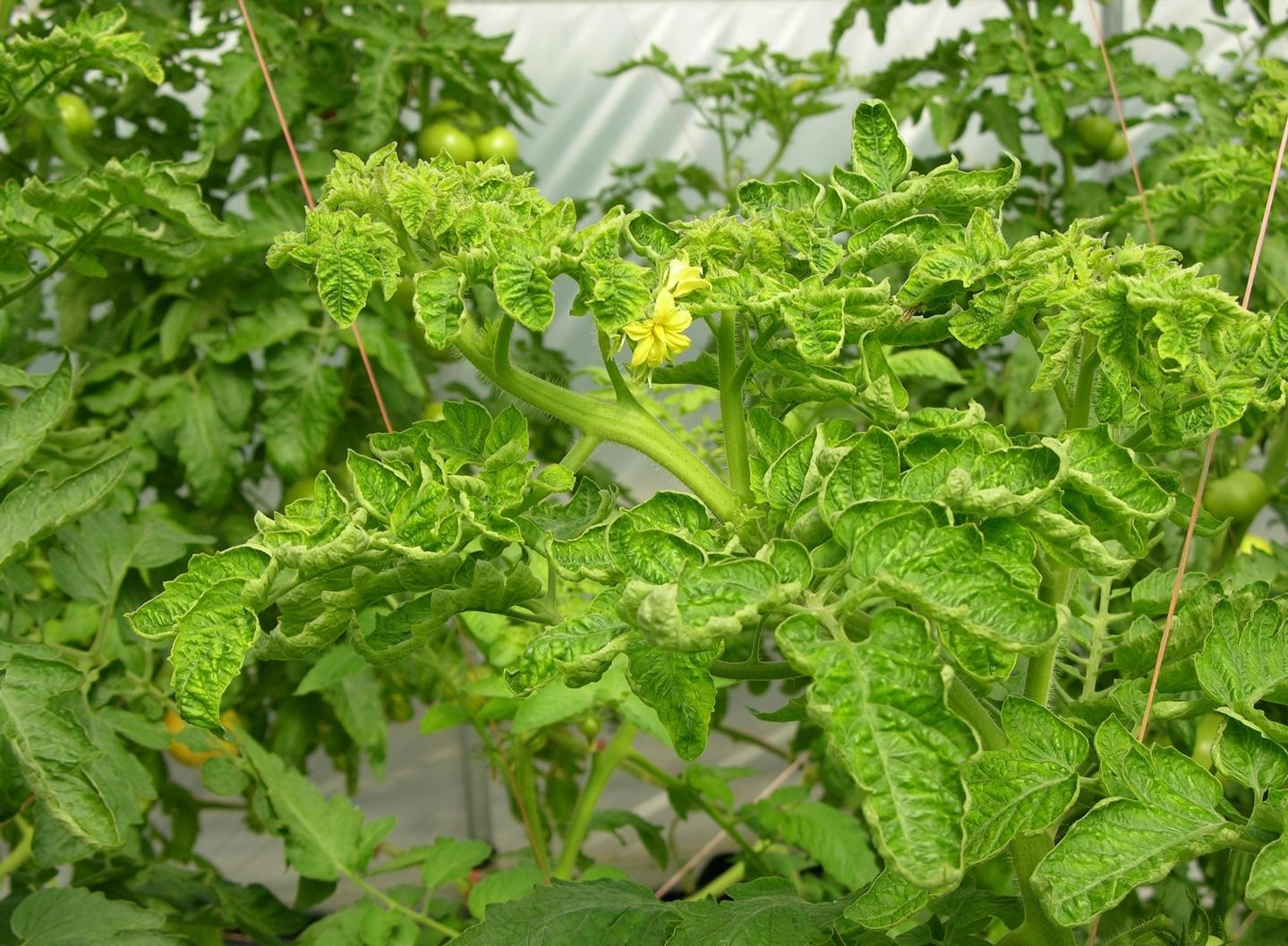
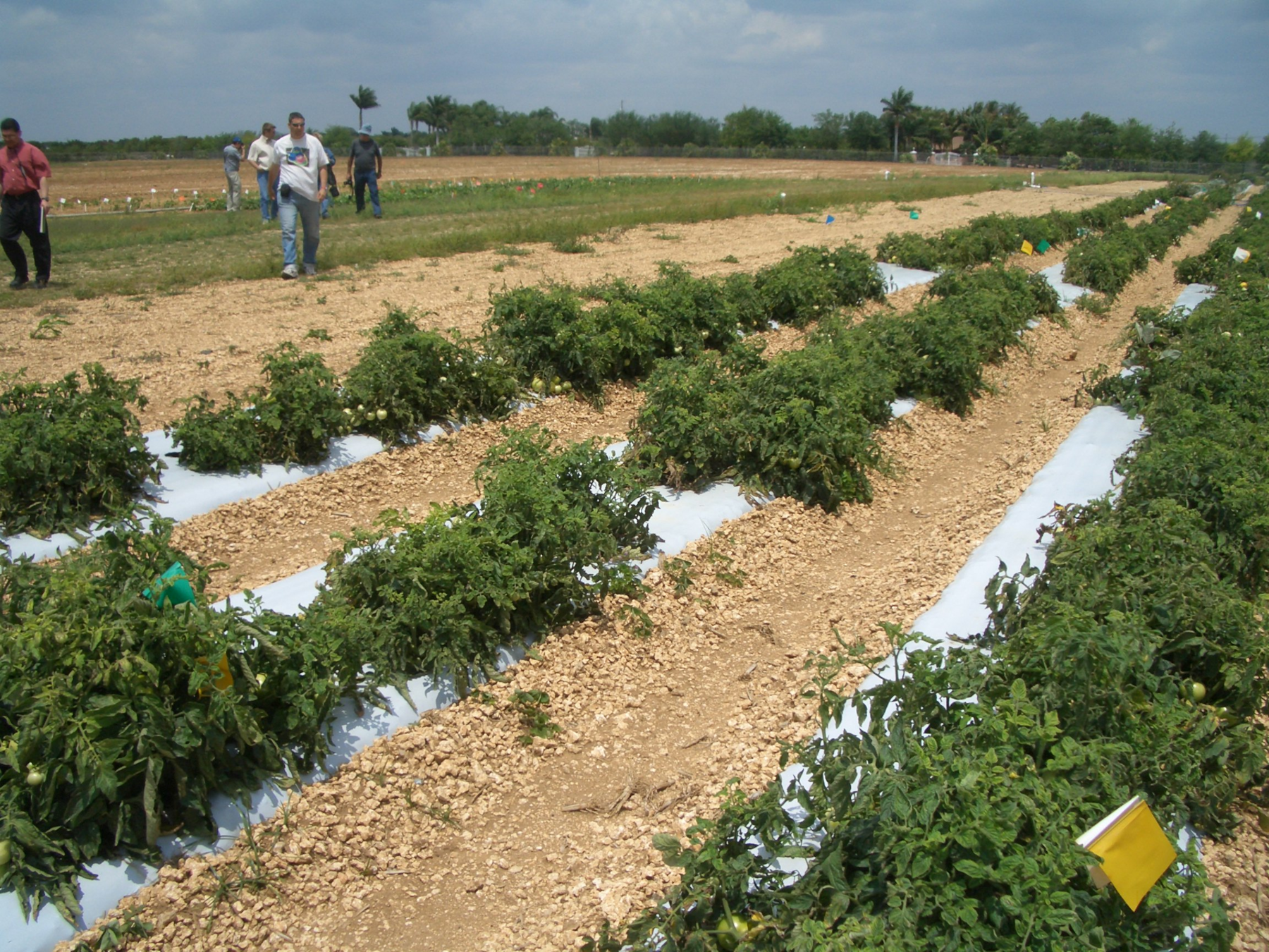
  • TYLCV Disease
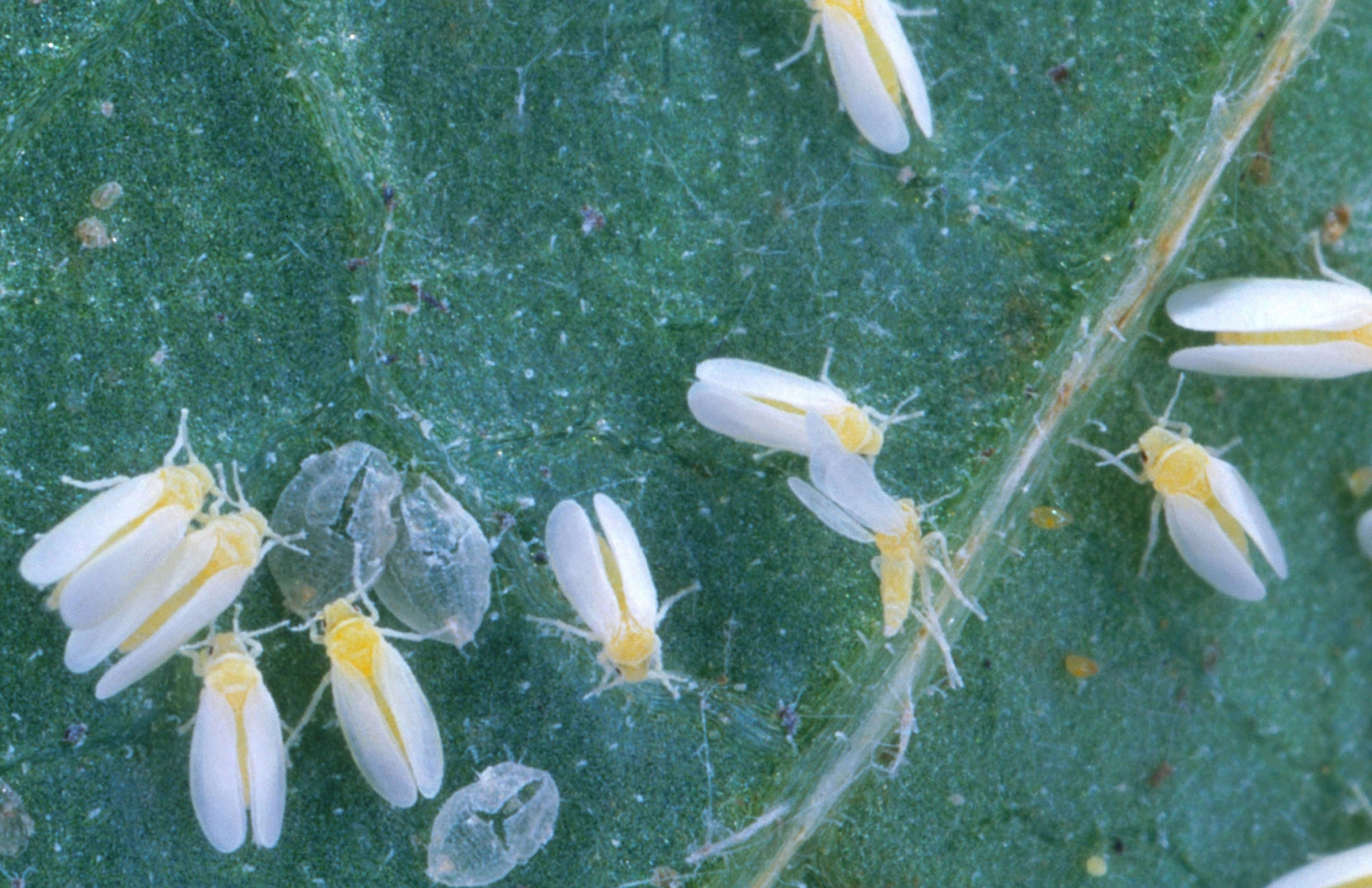
  • is spread by the insect whitefly (Bemisia tabaci)
  • How to Manage TYLCV?
  • Replanting infected plants suffers random fluctuations due to is leading identification because a yellow plant is not necessarily infected.               

  • The protocol to manage infected plants suggests replanting neighbors. Then naturally, a farmer could randomly replant a healthy plant instead of a latent one.
  • Thus strategies like fumigation with insecticide suffer random fluctuationsin their efficiency.

Controls

  • Replanting
  • Fumigation
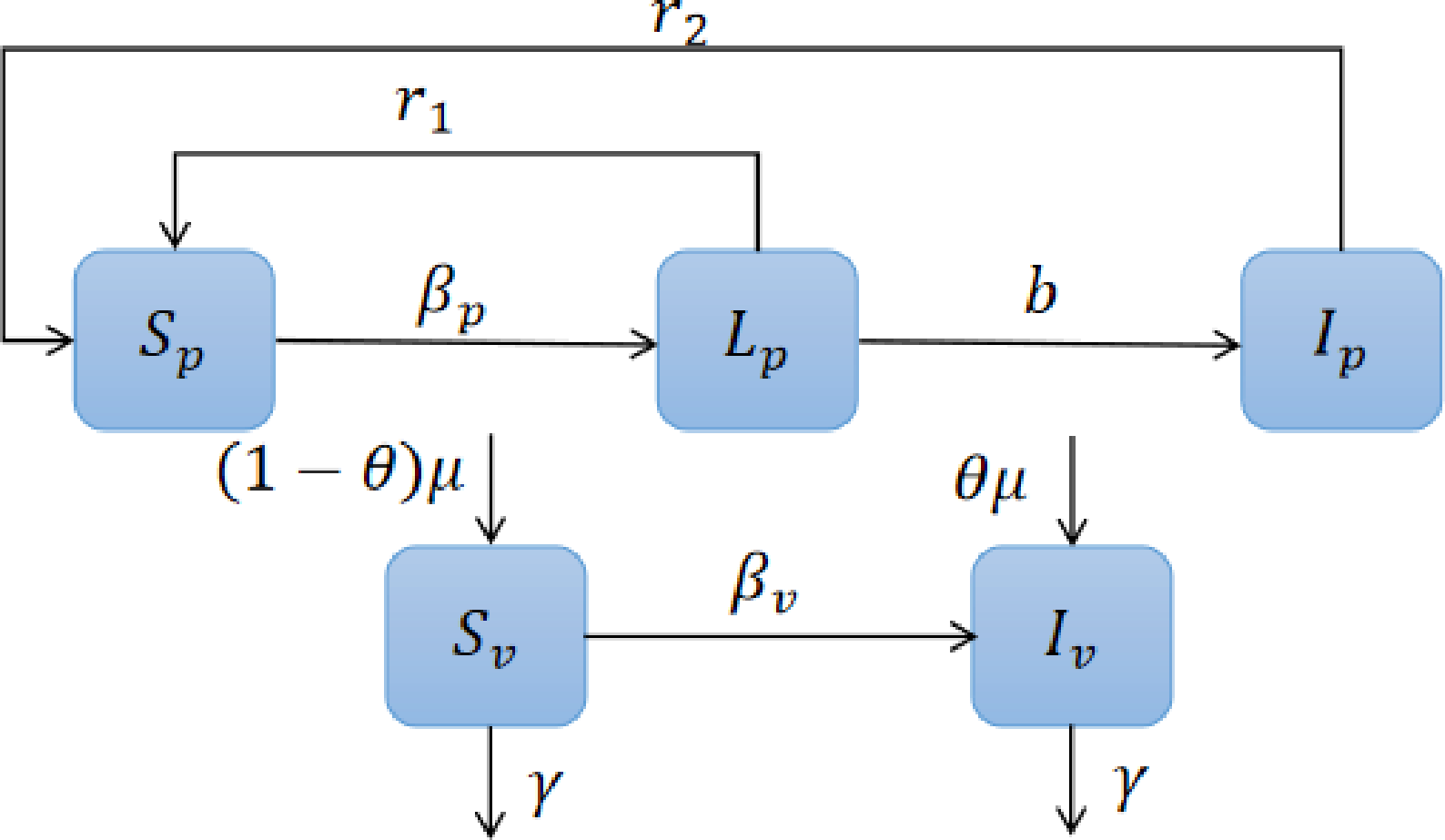
\begin{aligned} \dot{S_p} &= -\beta_p S_p I_v +\textcolor{blue}{r_1}L_p + \textcolor{blue}{r_2} I_p,\\ \dot{L_p} &= \beta_p S_p I_v -(b +\textcolor{blue}{r_1}) L_p,\\ \dot{I_p} &= b L_p - \textcolor{blue}{r_2} I_p,\\ \dot{S_v} &= -\beta_v S_v I_p - (\gamma +\textcolor{orange}{ \gamma_f}) S_v +(1-\theta)\mu,\\ \dot{I_v} &= \beta_v S_v I_p -(\gamma+\textcolor{orange}{\gamma_f}) I_v +\theta\mu. \end{aligned}
\begin{aligned} & \min_{\bar{u}(\cdot)\in \mathcal{U}_{x_0}[t_0,T]}J(u) \\ \text{Subject to} & \\ \dot{S_p} &= - \beta_p S_p I_v + \textcolor{blue}{(r_1 +u_1)} L_p + \textcolor{blue}{(r_2 + u_2)} I_p, \\ \dot{L_p} &= \beta_p S_p I_v -(b + \textcolor{blue}{(r_1 + u_1))} L_p, \\ \dot{I_p} &= b L_p - \textcolor{blue}{(r_2 + u_2)} I_p, \\ \dot{S_v} &= - \beta_v S_v I_p - (\gamma+ \textcolor{orange}{(\gamma_f + u_3)} ) S_v + (1-\theta)\mu, \\ \dot{I_v} &= \beta_v S_v I_p - (\gamma + \textcolor{orange}{(\gamma_f + u_3)}) I_v + \theta\mu, \\ &S_p(0) = S_{p_0}, L_p(0) = L_{p_0}, I_p(0) = I_{p_0}, \\ &S_v(0) = S_{v_0}, I_v(0) = I_{v_0}, u_i(t) \in [0, u_i ^ {max}]. \end{aligned}
\begin{aligned} J(u) &= \int_{0}^T \Big[A_1 I_p(t) + A_2 L_p(t) + A_3 I_v(t) + \sum^3_{i=1}c_i u_i(t)^2 \Big] dt, \end{aligned}

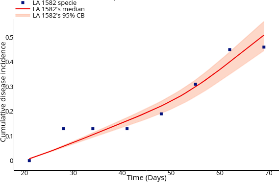
Performing parameter calibration using MCMC (Markov Chain Monte Carlo).

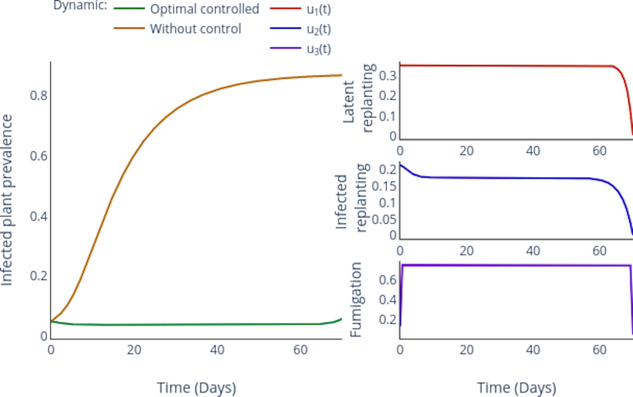
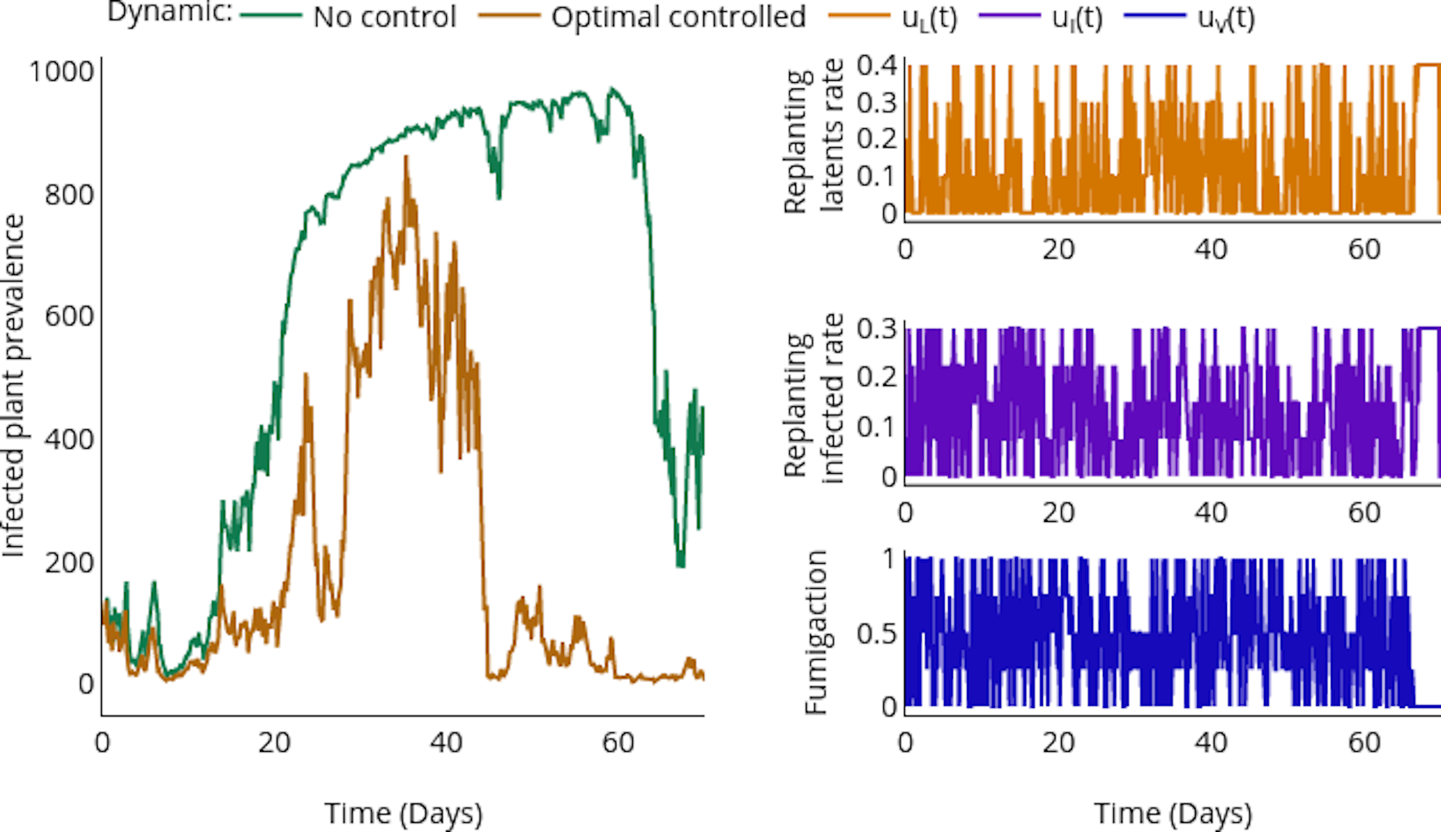
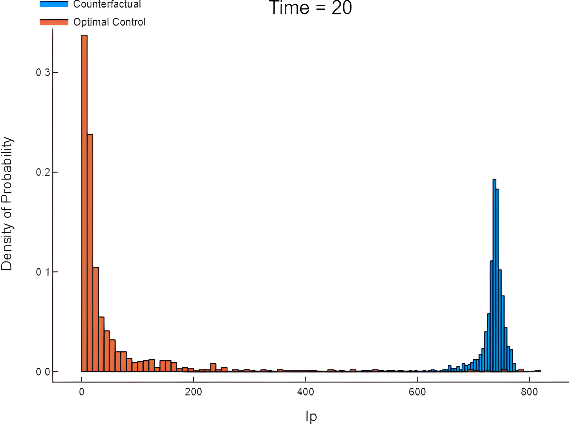
Simulation: Counterfactual vs Controlled.

\begin{aligned} \text{OCM}^T:& \\ & \min_{a_{\cdot} \in \mathcal{A}} c(x(\cdot), a(\cdot)) = \int_0 ^ T c_{0}(s, x(s)) ds + \int_0 ^ T c_1(s, a(s))ds \\ \text{s.t.}& \\ & \dot{x(t)} = F(x(t), \theta, a(t)), \qquad x(0)= x_0. \end{aligned}
x(t)

Spread Dynamics

Controller

a_t \in \mathcal{A}
\xi_t
\begin{aligned} \text{sto-OCM}^T:& \\ & \min_{a_{\cdot} \in \mathcal{A}} c(x(\cdot), a(\cdot)) = \textcolor{orange}{\mathbb{E}^{\pi}} \Big[ \int_0 ^ T c_{0}(s, x(s)) dW_s + \int_0 ^ T c_1(s, a(s))ds \Big] \\ \text{s.t.}& \\ & \dot{x(t)} = F( x(t), \theta, a(t), \textcolor{orange}{\xi_t} ), \qquad x(0)= x_0. \end{aligned}

SDEs, CTMC, Sto-Per

Data

Sto-Modelling

Control

Stochastic extension

\begin{aligned} \frac{d}{dt}x(t) = f(t,x(t)) & \rightsquigarrow dx(t) = f(t,x(t))dt + g(t,x(t))dB(t) \\ \alpha & \rightsquigarrow \alpha + P(x(t))\frac{dB(t)}{dt} \end{aligned}
\begin{aligned} \frac{dS_p}{dt} &= -\beta_p S_p \frac{I_v}{N_v} + \textcolor{blue}{r_1} L_p + \textcolor{blue}{r_2} I_p,\\ \frac{dL_p}{dt} &= \beta_p S_p \frac{I_v}{N_v} - (b + \textcolor{blue}{r_1}) L_p,\\ \frac{dI_p}{dt} &= b L_p - \textcolor{blue}{r_2} I_p,\\ \frac{dS_v}{dt} &= -\beta_v S_v \frac{I_p}{N_p} - (\gamma + \textcolor{orange}{\gamma_f}) S_v + (1-\theta)\mu,\\ \frac{dI_v}{dt} &= \beta_v S_v \frac{I_p}{N_p} - (\gamma + \textcolor{orange}{\gamma_f}) I_v +\theta\mu,\\ \end{aligned}
\begin{aligned} r_1 dt \rightsquigarrow r_1 dt + \sigma_L\frac{S_p}{N_p}dB_p(t), \\ r_2 dt \rightsquigarrow r_2 dt + \sigma_I\frac{S_p}{N_p} dB_p(t), \\ \gamma_f dt \rightsquigarrow \gamma_f dt + \sigma_v dB_v(t). \end{aligned}
\begin{aligned} d S_p &= \left( -\beta_p S_p \frac{I_v}{N_v} + \textcolor{blue}{r_1} L_p + \textcolor{blue}{r_2} I_p \right)dt + \textcolor{blue}{\frac{S_p(\sigma_L L_p + \sigma_I I_p)}{N_p}} dB_p(t), \\ dL_p &= \left( \beta_p S_p \frac{I_v}{N_v} - (b + \textcolor{blue}{r_1}) L_p \right) dt - \textcolor{blue}{\sigma_L \frac{S_p L_p}{N_p}} dB_p(t), \\ d I_p &= \left( b L_p - \textcolor{blue}{r_2} I_p \right) dt - \textcolor{blue}{\sigma_I \frac{S_pI_p}{N_p}} dB_p(t), \\ dS_v &= \left( -\beta_v S_v \frac{I_p}{N_p} - (\gamma + \textcolor{orange}{\gamma_f}) S_v + (1-\theta) \mu \right)dt - \textcolor{orange}{\sigma_v S_v} dB_v(t), \\ d I_v &= \left( \beta_v S_v \frac{I_p}{N_p} - (\gamma + \textcolor{orange}{\gamma_f}) I_v + \theta \mu \right) dt - \textcolor{orange}{\sigma_v I_v} dB_v(t). \end{aligned}

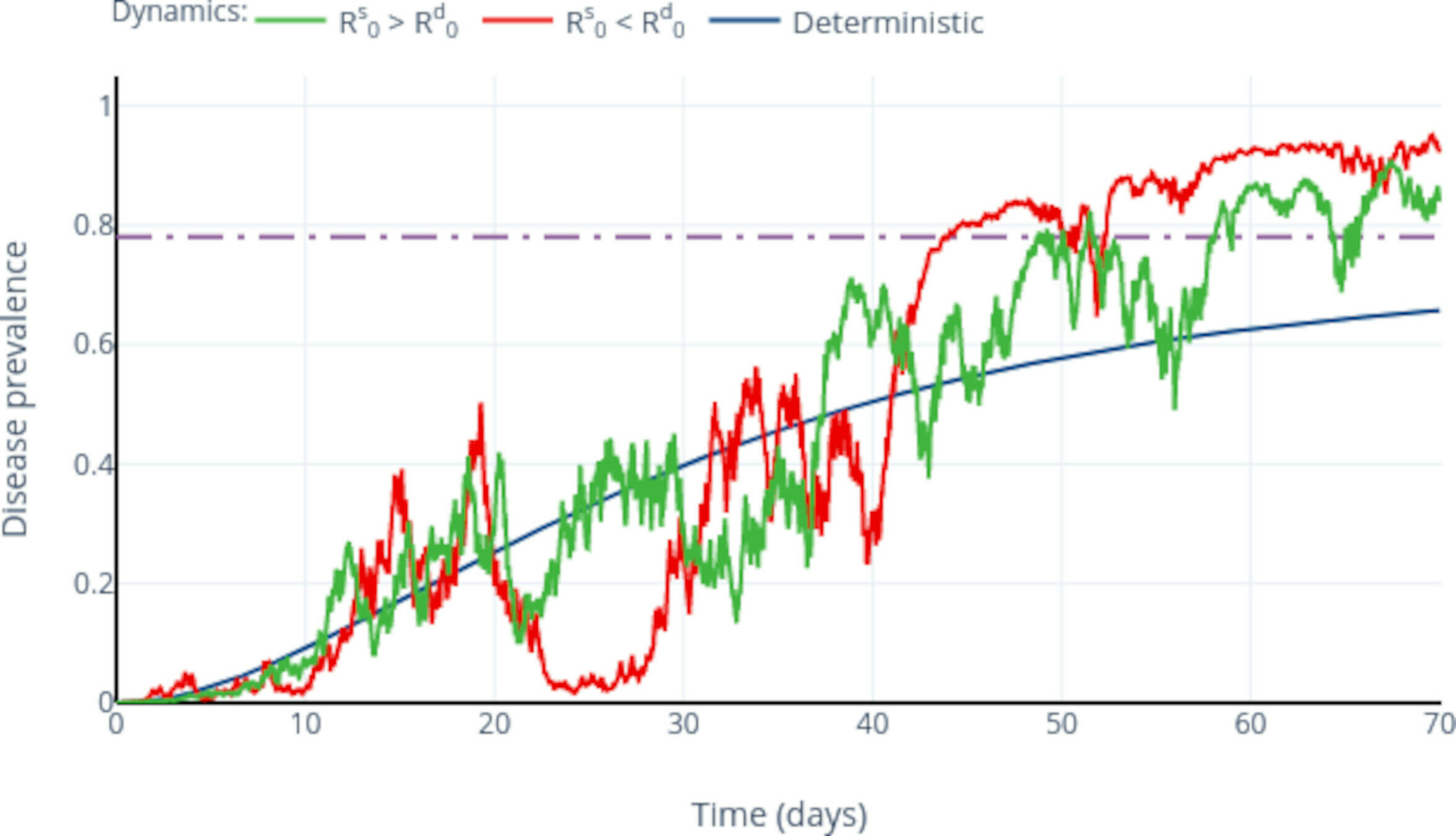
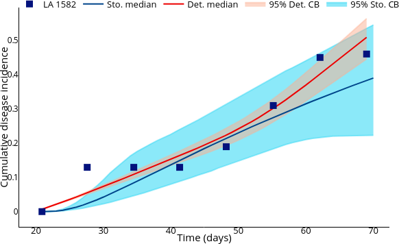
Enhancing parameter calibration through noise

\begin{aligned} dx(t) &= f(t, x(t), \textcolor{orange}{u(t)})dt + g(t, x(t), u(t)) dW(t),\\ x(0) &= x_0 \in \mathbb{R}^n, \\ \\ J(u(\cdot)) &= \mathbb{E} \left\{ \int^T_0 c(t,x(t),u(t)) dt + h(x(T))\right\}. \end{aligned}
\begin{aligned} &J(\bar{\pi}) = \inf_{\pi \in\, \mathcal{U}[0,T]} J(\pi)\\ \text{Suject to}&\\ dx(t) &= f(t, x(t), u(t))dt + g(t, x(t), u(t)) dW(t),\\ x(0) &= x_0 \in \mathbb{R}^n, \end{aligned}
\begin{aligned} \forall t & \in[0,T], \ x, \ \hat{x} \in \mathbb{R}^n, \ u \in U, \\ &|\varphi(t,x,u) - \varphi(t, \hat{x},u)|\leq L|x-\hat{x}|, \end{aligned}
\begin{aligned} f:[0,T] \times \mathbb{R} ^ n \times U &\to \mathbb{R}^n, \\ g:[0,T] \times\mathbb{R} ^ n \times U &\to \mathbb{R}^{n\times m}, \\ c:[0,T] \times\mathbb{R} ^ n \times U &\to \mathbb{R}, \\ h:\mathbb{R}^n \to \mathbb{R}& \end{aligned}
\begin{aligned} (s,y) \in [0,T) &\times \mathbb{R}^n, \\ V(s,y) &= \inf_{ u(\cdot) \in \mathcal{U} [s,T]} J(s, y; u(\cdot) ), \\ V(T,y) &= h(y), \qquad \forall y\in \mathbb{R}^n, \end{aligned}
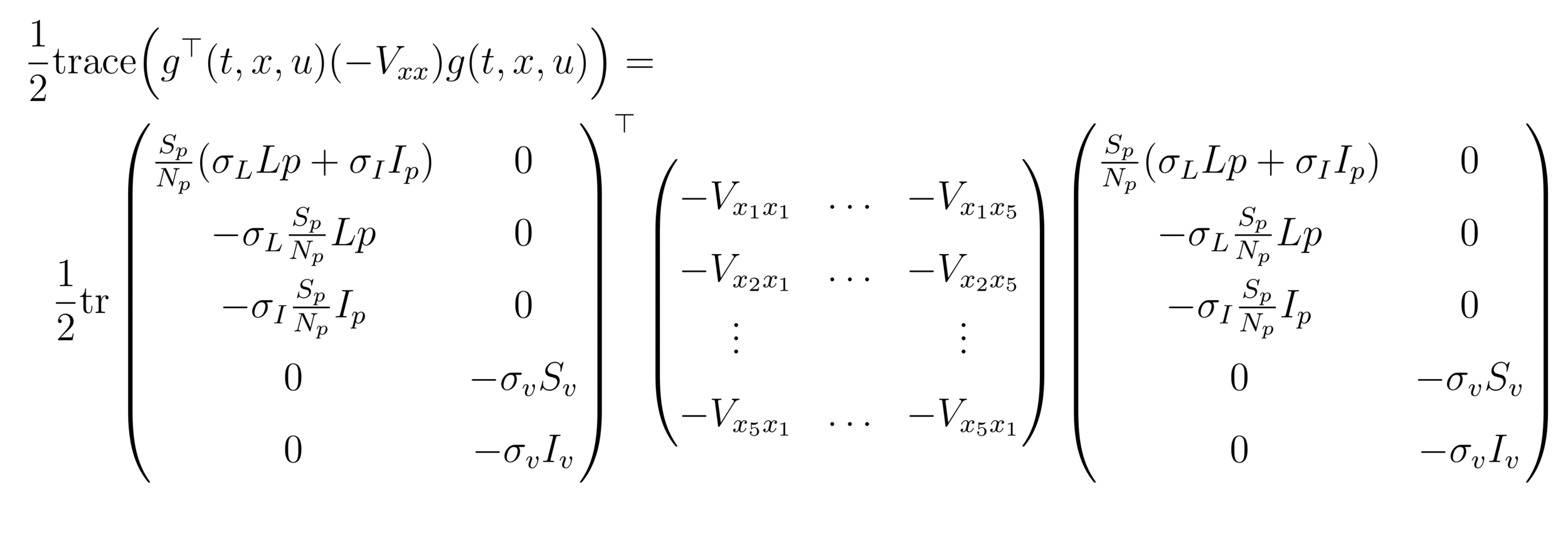
\begin{aligned} & -V_t + \sup_{u \in U} H_G (t ,x, u, -V_x, -V_{xx})=0, (t,x) \in [0,T)\times\mathbb{R}^n, \\ & V \Big|_{t=T} = h(x), \qquad x\in \mathbb{R} ^ n, \\ & H_G(t,x,u,p,P) = \langle p, f(t,x,u) \rangle - c(t,x,u) \\ &+\dfrac{1}{2} \mathtt{trace}\Big( g^\top(t,x,u)Pg(t,x,u)\Big) \\ & = H_{det}(t,u,x,p) +\dfrac{1}{2} \mathtt{trace}\Big( g^\top(t,x,u)Pg(t,x,u)\Big) \end{aligned}
\begin{aligned} \forall (t,u) & \in [0,T]\times U \\ &|\varphi(t,0,u)|\leq L \end{aligned}

OPC:

Value Function

HJB

\begin{aligned} dx(t) &= f(t, x(t), \textcolor{orange}{u(t)})dt + g(t, x(t), u(t)) dW(t),\\ x(0) &= x_0 \in \mathbb{R}^n, \\ J(u(\cdot)) &= \mathbb{E} \left\{ \int^T_0 c(t,x(t),u(t)) dt + h(x(T))\right\}. \end{aligned}
\begin{aligned} J(u) = \mathbb{E}\int_{0}^{T} & \Bigg[ A_1 I_p(t) + A_2 L_p(t) + A_3 I_v (t) \\ & + c_1 u ^ 2_1(t) + c_2 u ^ 2_2(t) + c_3 u ^ 2_3(t) \Bigg] dt, \end{aligned}
\begin{aligned} &\qquad\qquad\qquad\qquad\min_{u\in \mathcal{U}[0,T]} J(u) \\ &\qquad \text{subject to } \\ &dS_p = \left( -\beta_pS_p\frac{I_v}{N_v}+(r_1 +u_1) L_p + (r_2 + u_2)L_p \right)dt \\ &+ \frac{S_p}{N_p}\left( \sigma_L L_p+\sigma_I I_p \right)dB_p,\\ &dL_p = \left( \beta_pS_p\frac{I_v}{N_v}-(b+r_1 +u_1)L_p \right)dt -\sigma_L\frac{S_p}{N_p}L_pdB_p, \\ &dI_p = \left( b L_p - (r_2 + u_2) I_p \right)dt - \sigma_I\frac{S_p}{N_p}I_p dB_p, \\ &dS_v = \left( -\frac{\beta_v}{N_p}S_vI_p -(\gamma +\gamma_f+ u_3) S_v + (1-\theta)\mu\right)dt -\sigma_v S_vdB_v, \\ &dI_v = \left( \frac{\beta_v}{N_p}S_vI_p - (\gamma +\gamma_f+u_3) I_v +\theta \mu \right) dt - \sigma_v S_v dB_v. \end{aligned}
\begin{aligned} V(s,x) = \inf_{u(\cdot) \in \mathcal {U}[s,T]} &\mathbb{E} \Bigg\{ \int_{s}^{T} \Big[ A_1 I_p(t) + A_2 L_p(t) + A_3 I_v (t) \\ & + c_1 u ^ 2_1(t) + c_2 u ^ 2_2(t) + c_3 u ^ 2_3(t) \Big] dt \Bigg\} \end{aligned}
\begin{aligned} &-V_t + \sup_{u \in U} H_G(t, x, u, -V_x, -V_{xx})=0 \end{aligned}
\begin{aligned} H_G(t,x,u,p,P) &= \langle p, f(t,x,u) \rangle - c(t,x,u) \\ &+\dfrac{1}{2} \mathtt{trace}\Big( g^\top(t,x,u)Pg(t,x,u)\Big) \end{aligned}
\begin{aligned} H_{det} &(t,u,x,-V_x) = A_1I_v+A_2L_p+A_3I_v +\sum_{i=1}^{3}c_iu_i^2\\ &-V_{x_1}(-\beta_p S_p I_v +(r_1 +u_1)L_p + (r_2 + u_2) I_p)\\ & -V_{x_2}(\beta_p S_p I_v-(b +r_1 + u_1)L_p)\\ &-{V_{x_3}}(b L_p - (r_2 + u_2) I_p)\\ &-V_{x_4}(-\beta_v S_v I_p - (\gamma+\gamma_f+u_3) S_v +(1-\theta)\mu)\\ &-V_{x_5}(\beta_v S_v I_p -(\gamma+\gamma_f+u_3) I_v+\theta\mu). \end{aligned}
HJB (Dynamic Programming)
  • Course of dimensionality
\approx \ \mathtt{HJB}
HJB (Neuro-Dynamic Programming)

Bertsekas, Dimitri P.

Abstract dynamic programming.

Athena Scientific, Belmont, MA, 2013. viii+248 pp.

ISBN:978-1-886529-42-7

ISBN:1-886529-42-6

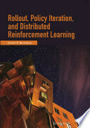
Bertsekas, Dimitri P.

Rollout, policy iteration, and distributed reinforcement learning.

Revised and updated second printing

Athena Sci. Optim. Comput. Ser.

Athena Scientific, Belmont, MA, [2020], ©2020. xiii+483 pp.

ISBN:978-1-886529-07-6

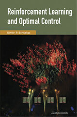
Reinforcement learning and optimal control

Bertsekas, Dimitri P.

Athena Sci. Optim. Comput. Ser.

Athena Scientific, Belmont, MA, 2019, xiv+373 pp.

ISBN: 978-1-886529-39-7

\frac{dx_{t}}{dt} =f(x_{t} ,a_{t})

Agent

a_t\in \mathcal{A}
C_t
x_t
\begin{aligned} %C_{t+1} &= C(x_{t}, a_{t}) \\ %\Phi_{t+1}^{h}(x_t,a_t) &= x_t + f(x_{t} ,a_{t})\varphi(h,\theta) \end{aligned}

Agent

R_{t+1}
x_{t+1}
x_0,a_0,R_1,
a_t\in \mathcal{A}(x_t)

action

state

x_{t}

reward

R_{t}
x_0, a_0, R_1, x_1, a_1, R_2, \cdots, x_t, a_t, R_{t+1} \cdots, x_{T-1}, a_{T-1}, R_T, x_T
G_t := R_{t+1} + \cdots + R_{T-1} + R_{T}
\begin{aligned} G_t &:= R_{t+1} + \gamma R_{t+2} + \gamma^2 R_{t+3}+ \cdots \\ &= \sum_{k=0} \gamma^{k} R_{t+1+k}, \qquad \gamma \in [0,1] \end{aligned}
G_t := R_{t+1} + \cdots + R_{T-1} + R_{T}
\begin{aligned} G_t &:= R_{t+1} + \gamma R_{t+2} + \gamma^2 R_{t+3}+ \cdots \\ &= \sum_{k=0}^{\infty} \gamma^{k} R_{t+1+k}, \qquad \gamma \in [0,1] \end{aligned}
p(s^{\prime},r | s, a) := \mathbb{P}[x_t=s^{\prime}, R_{t}=r | x_{t-1}=s, a_t=a]
\begin{aligned} r(s, a) &:= \mathbb{E}[ R_t | S_{t-1}=s, a_{t}=a ] \\ &= \sum_{r\in \mathcal{R}} r \sum_{s^{\prime}\in S} p(s^{\prime}, r | s, a) \end{aligned}
\begin{aligned} G_t &:= R_{t+1} + \gamma R_{t+2} + \cdots + \gamma^{T-t-1} R_{T} \\ &=\sum_{k=t+1}^{T} \gamma^{k-t-1} R_k \end{aligned}

Discounted return

Total return

\begin{aligned} v_{\pi}(s) &:= \mathbb{E}_{\pi} [G_t | x_t = s] \\ &= \mathbb{E}_{\pi} \left[ \sum_{k=0}^{\infty} \gamma^{k} R_{t+k+1} \big| x_t =s \right] \end{aligned}
\pi(a|s):= \mathbb{P}[a_t = a|x_t=s]
\begin{aligned} v_{\pi}(s) &:= \mathbb{E}_{\pi} [G_t | x_t = s] \\ &= \mathbb{E}_{\pi} \left[ \sum_{k=0}^{\infty} \gamma^{k} R_{t+k+1} \big| x_t =s \right] \\ & = \mathbb{E}_{\pi} \left[ R_{t+1} + \gamma G_{t+1} | x_t = s \right] \\ &= \sum_{a} \pi(a |s) \sum_{s^{\prime}, r} p(s^{\prime},r | s, a) \left[ r + \gamma \mathbb{E}_{\pi}[G_{t+1} | x_{t+1}=s^{\prime}] \right] \\ &= \sum_{a} \pi(a |s) \sum_{s^{\prime}, r} p(s^{\prime},r | s, a) \left[ r + \gamma v_{\pi}(s^{\prime}) \right] \end{aligned}
\begin{aligned} v_{*}(s) &:= \max_{\pi} v_{\pi}(s) \\ &= \max_{a\in \mathcal{A}(s)} \mathbb{E}_{\pi_{*}} \left[ \sum_{k=0}^{\infty} \gamma^{k} R_{t+k+1} \big| x_t =s \right] \\ & = \max_{a\in \mathcal{A}(s)} \mathbb{E}_{\pi} \left[ R_{t+1} + \gamma G_{t+1} | x_t = s \right] \\ &= \max_{a\in \mathcal{A}(s)} \sum_{a} \pi(a |s) \sum_{s^{\prime}, r} p(s^{\prime},r | s, a) \left[ r + \gamma \mathbb{E}_{\pi}[G_{t+1} | x_{t+1}=s^{\prime}] \right] \\ &= \max_{a\in \mathcal{A}(s)} \sum_{a} \pi(a |s) \sum_{s^{\prime}, r} p(s^{\prime},r | s, a) \left[ r + \gamma v_{\pi}(s^{\prime}) \right] \end{aligned}
x_0, a_0, R_1, x_1, a_1, R_2, \cdots, x_t, a_t, R_{t+1} \cdots, x_{T-1}, a_{T-1}, R_T, x_T
\begin{aligned} x_{t_{n+1}} & = x_{t_n} + F(x_{t_n}, \theta, a_0) \cdot h, \quad x_{t_0} = x(0), \\ \text{where: }& \\ t_n &:= n \cdot h, \quad n = 0, \cdots, N, \quad t_{N} = T. \end{aligned}
\begin{aligned} &\min_{a_{0} \in \mathcal{A}_0} c(x_{\cdot}, a_0):= c_1(a_0)\cdot T + \sum_{n=0}^{N-1} c_0(t_n, x_{t_n}) \cdot h \\ \text{ s.t.} & \\ & x_{t_{n+1}} = x_{t_n} + F(x_{t_n}, \theta, a_0) \cdot h, \quad x_{t_0} = x(0), \\ \text{where: }& \\ t_n &:= n \cdot h, \quad n = 0, \cdots, N, \quad t_{N} = T. \end{aligned}

Modeling a traffic light warning system for acute respiratory infections as an optimal control problem

Saul Diaz Infante Velasco

Adrian Acuña Zegarra

Jorge Velasco Hernandez

sauldiazinfante@gmail.com

Introduction

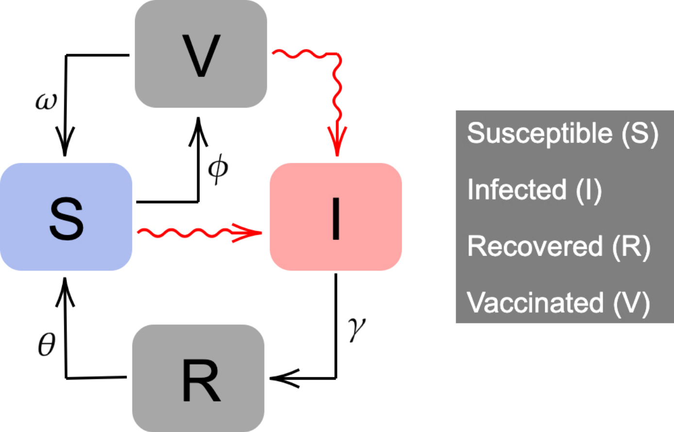
We propose an extension of the classic Kermack-McKendrick mathematical model. 𝑁(𝑡) is constant and is split into four compartments:

  • susceptible (𝑆(𝑡)),
  • infected (𝐼(𝑡)),
  • recovered (𝑅(𝑡)),
  • and vaccinated (𝑉 (𝑡)).

Susceptible individuals can become infected when interacting with an infectious individual. After a period of time (1∕𝛾), infected people recover. Recovered people lose their natural immunity after a period of time 1∕𝜃.

C_k(t^*) = 1 - \left(1 - \frac{I(t^*)}{N(t^*)}\right)^k

Risk index

Another closely related index that has been used to monitor and evaluate the development of ARI is the event gathering risk, developed by Chande (2020).

Chande, A., Lee, S., Harris, M. et al. Real-time, interactive website for US-county-level COVID-19 event risk assessment. at Hum Behav, 1313–1319 (2020). https://doi.org/10.1038/s41562-020-01000-9

\begin{aligned} S' =& \mu N - \lambda(t)S - (\phi + \mu) S + \omega V + \theta R \\ I' =& \lambda(t) (S + (1 - \sigma)V) - (\gamma + \mu) I \\ V' =& \phi S - (1 - \sigma) \lambda(t)V - (\omega + \mu) V \\ R' =& \gamma I - (\theta + \mu) R \end{aligned}
\begin{aligned} C^{\prime} =& k (1 - C)^{\left(1 - \frac{1}{k}\right)} \left(1 - (1 - C)^{\frac{1}{k}}\right) \\ & \times \left( \beta(t) (1 - C(t)) (S + (1 - \sigma)V) \frac{1}{N} - (\gamma + \mu) \right). \end{aligned}
\begin{aligned} \beta(t) & = \left( 1 + a \cos \left( \frac{2\pi}{365} t \right) \right) \beta_0 \\ \lambda(t) & = \beta(t) (1 - C(t)) \frac{I(t)}{N} \end{aligned}
# MODEL FORMULATION
C(t) = 1 - \left(1 - \frac{I(t)}{N}\right)^k

Risk index

gives the probability of finding at time t an infected person in a group of k individuals.

\begin{aligned} C' =& k (1 - C)^{\left(1 - \frac{1}{k}\right)} \left(1 - (1 - C)^{\frac{1}{k}}\right) \\ & \times \left( \beta(t) (1 - C(t)) (S + (1 - \sigma)V) \frac{1}{N} - (\gamma + \mu) \right) \end{aligned}
\begin{aligned} s^{\prime} &= \mu - \hat{\lambda}(t)s - (\phi + \mu) s + \omega v + \theta r \\ i^{\prime} &= \hat{\lambda}(t) (s + (1 - \sigma)v) - (\gamma + \mu) i \\ v^{\prime} &= \phi s - (1 - \sigma) \hat{\lambda}(t)v - (\omega + \mu) v \\ r^{\prime} &= \gamma i - (\theta + \mu) r \\ C^{\prime} &= k (1 - C)^{\left(1 - \frac{1}{k}\right)} \left( 1 - (1 - C)^{\frac{1}{k}} \right) \\ & \times \left( \beta(t) (1 - C(t)) (s + (1 - \sigma) v) - (\gamma + \mu) \right) \end{aligned}

# REPRODUCTIVE NUMBER

s = \frac{S}{N}; \quad i = \frac{I}{N}; \quad v = \frac{V}{N}; \quad r = \frac{R}{N}

Normalization

\begin{aligned} \Omega = \Big \{ & (s, i, v, r, C)\in \mathbb{R}^5_+ : \\ & 0\leq C\leq 1, \\ & 0 \leq y \leq 1, \forall y \in \{s, i, v, r \}, \\ & s + i + v + r = 1 \Big \} \end{aligned}

Invariance

\mathcal{R}_0 = \frac{\beta_0(1 - C^*)(s^* + (1 - \sigma)v^*)}{(\gamma + \mu)}

Basic Reproductive number

\begin{aligned} s^* &= \frac{\omega + \mu}{\phi + \omega + \mu} \\ v^* &= \frac{\phi}{\phi + \omega + \mu} \\ C^* &= 0 \end{aligned}

FDE

Effective reproduction number

\mathcal{R}_t = \frac{\beta(t)(1 - C(t))(s(t) + (1 - \sigma)v(t))}{(\gamma + \mu)}
# Light Traffic Policies and  Optimal Control
x(t)^\top:= (s(t), i(t),v(t),r(t), C(t))
a(t_k) \xrightarrow{\varphi}
A(\xi):= \Big \{green, yellow, orange, red \Big\}
(u_{\beta}^{4}, u_k^{4})
(u_{\beta}^{1}, u_k^{1})
(u_{\beta}^{3}, u_k^{3})
(u_{\beta}^{2}, u_k^{2})
  • A decision-maker can apply a strategy from a finite set of actions.
  • The set of actions implies a particular effect accordingly to the light semaphore.
  • We describe this effect by modulating the transmission rate and size of gathering :
\beta(t),\ k.
  • A decision-maker can apply a strategy from a finite set of actions.
  • The set of actions implies a particular effect accordingly to the light semaphore.
  • We describe this effect by modulating the transmission rate and size of gathering.
\begin{aligned} \widehat{\lambda}(u_{\beta}, T_j):= & \beta(t)(1 - u_{\beta}) (1 - C(t)) y(t) \\ k(u_k, T_j):= & (1 - u_k) k \end{aligned}
\begin{aligned} x^{\prime} =& \mu - \widehat{\lambda}(u_{\beta}, t) x - (\phi + \mu) x + \omega v + \theta z \\ y^{\prime} =& \widehat{\lambda}(u_{\beta}, t) (x + (1 - \sigma)v) - (\gamma + \mu) y \\ v^{\prime} =& \phi x - (1 - \sigma) \widehat{\lambda}(u_{\beta}, t) v - (\omega + \mu) v \\ z^{\prime} =& \gamma y - (\theta + \mu) z \\ C^{\prime} =& k(u_k, T_j) (1 - C) ^ { \left( 1 - \frac{1}{k(u_k, T_j)} \right) } \left( 1 - (1 - C) ^ \frac{1}{k(u_k, T_j)} \right) \\ & \times \left[ \beta(t) (1 - u_{\beta}) (1 - C(t)) (x + (1 - \sigma) v) - (\gamma + \mu) \right] \end{aligned}
T_i
T_{i+1}
T_{i-1}
\overbrace{\text{decision period}}^{p_j := t_j - t_{j-1}}
\underset{ \substack{ j \in A \\ A:=\{\text{green, yellow, orange, red} \} } } %} { J \left( \xi^{[p_i]}, u_{\beta} ^{[j]}, u_k^{[j]} \right) } := \underbrace{ \int_{0}^T a_I y(s) }_{YLD} ds + \underbrace{ \int_{0}^T a_C C(s) + a_{\beta} u_{\beta}^2(s) + a_k u_k^2(s) }_{ \substack{ \text{political and economic} \\ \text{implications} } } ds.
\beta \rightsquigarrow \beta (1 -u_{\beta})
k \rightsquigarrow k (1 - u_{k})
\underset{ \substack{ j \in A \\ A:=\{\text{green, yellow, orange, red} \} } } %} { J \left( \xi^{[p_i]}, u_{\beta} ^{[j]}, u_k^{[j]} \right) } := \underbrace{ \int_{0}^T a_I y(s) }_{YLD} ds + \underbrace{ \int_{0}^T a_C C(s) + a_{\beta} u_{\beta}^2(s) + a_k u_k^2(s) }_{ \substack{ \text{political and economic} \\ \text{implications} } } ds.
  • The decision maker only chooses the strategy from a finite set of actions--as mentioned above-- and according to the light traffic protocol. Thus, the controller decides which color from the plausible light-traffic actions for the next period.
  • The corresponding authorities periodically meet every few weeks and make a decision.
  • The decision taken minimizes the functional J subject to the mentioned dynamics.


Hypothesis

T_i
T_{i+1}
T_{i-1}
\overbrace{\text{decision period}}^{p_j := t_j - t_{j-1}}

(OCP) Decide in each stage (a week), the light color that minimize functional cost J

\begin{aligned} \beta(t) := & \left( 1 + a \cos \left( \frac{2\pi}{365} t \right) \right) \beta_0 \\ \widehat{\lambda}(u_{\beta}, t_j):= & \beta(t)(1 - u_{\beta}) (1 - C(t)) i(t) \\ k(u_k, t_j):= & (1 - u_k) k \end{aligned}
\underset{ \substack{ j \in A \\ A:=\{\text{green, yellow, orange, red} \} } } { \min } J \left( \xi^{[p_i]}, u_{\beta} ^ {[j]}, u_k ^ {[j]} \right) := \underbrace{ \int_{T_{i-1}} ^ {T_{i}} a_I i(s) }_{YLD} ds + \underbrace{ \int_{T_{i-1}} ^{T_{i}} a_C C(s) + a_{\beta} u_{\beta}^2(s) + a_k u_k ^ 2(s) }_{ \substack{ \text{political and economic} \\ \text{implications} } } ds.

subject to:

\begin{aligned} s^{\prime} &= \mu - \hat{\lambda}(t)s - (\phi + \mu) s + \omega v + \theta r \\ i^{\prime} &= \hat{\lambda}(t) (s + (1 - \sigma)v) - (\gamma + \mu) i \\ v^{\prime} &= \phi s - (1 - \sigma) \hat{\lambda}(t)v - (\omega + \mu) v \\ r^{\prime} &= \gamma i - (\theta + \mu) r \\ C^{\prime} &= k (1 - C)^{\left(1 - \frac{1}{k}\right)} \left( 1 - (1 - C)^{\frac{1}{k}} \right) \\ & \times \left( \beta(t) (1 - C(t)) (s + (1 - \sigma) v) - (\gamma + \mu) \right) \end{aligned}

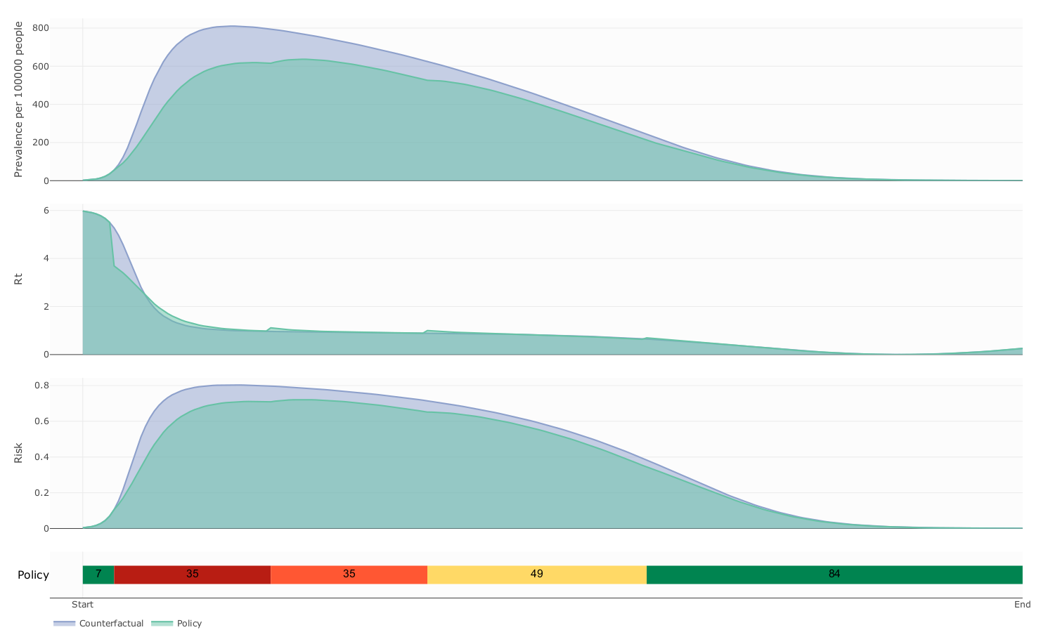
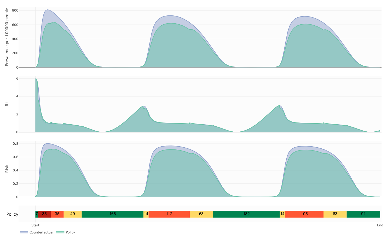
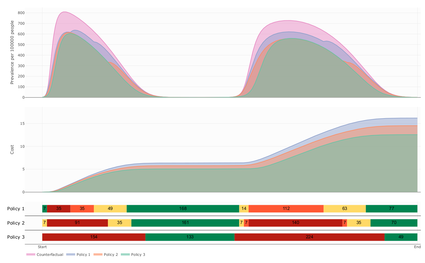
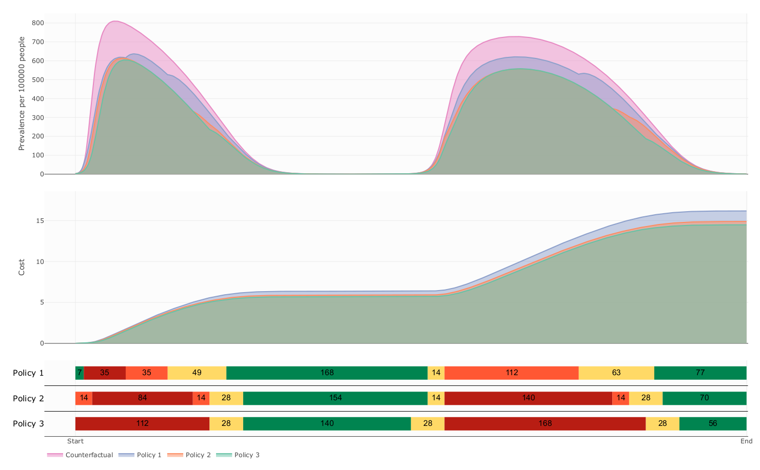
Counterfactual vs controlled dynamics

Counterfactual vs controlled dynamics

Counterfactual vs controlled dynamics

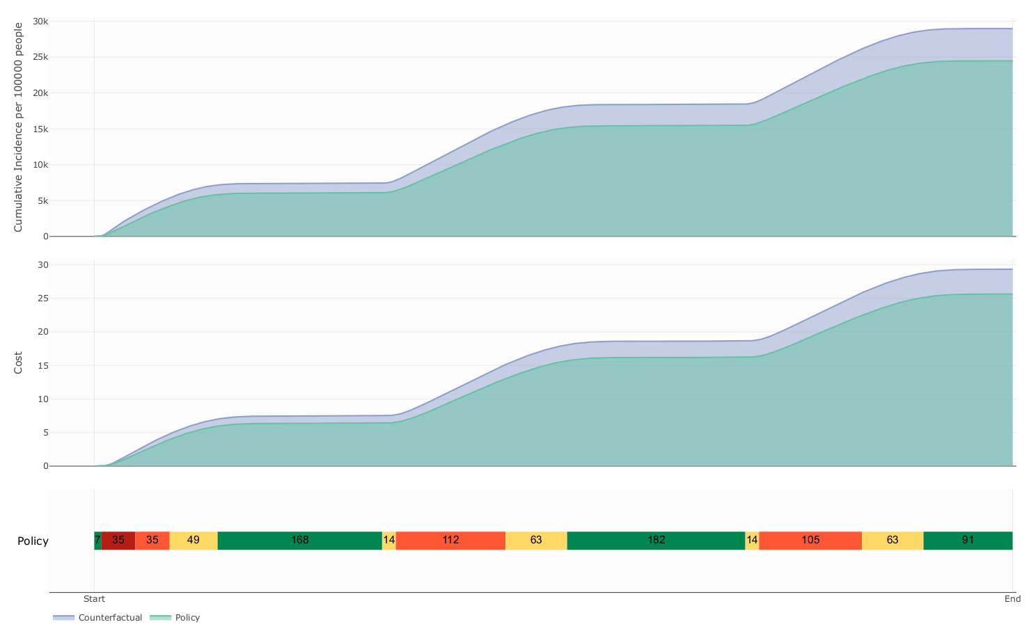
The influence of mobility restriction expenses over prevalence and cost 

\underset{ \substack{ j \in A \\ A:=\{\text{green, yellow, orange, red} \} } } { J \left( \xi^{[p_i]}, u_{\beta} ^ {[j]}, u_k ^ {[j]} \right) } := % \int_{T_{i-1}} ^ {T_{i}} a_I i(s) + a_C C(s) ds + \int_{T_{i-1}} ^{T_{i}} a_{\beta} u_{\beta}^2(s) + a_k u_k ^ 2(s) ds.

Expenses

due to mobility restrictions

a_{\beta} \searrow

The influence of decision period span over prevalence and cost 

\underset{ \substack{ j \in A \\ A:=\{\text{green, yellow, orange, red} \} } } { J \left( \xi^{[p_i]}, u_{\beta} ^ {[j]}, u_k ^ {[j]} \right) } := % \int_{T_{i-1}} ^ {T_{i}} a_I i(s) + a_C C(s) ds + \int_{T_{i-1}} ^{T_{i}} a_{\beta} u_{\beta}^2(s) + a_k u_k ^ 2(s) ds.
\underbrace{p_i:=T_{i+1} - T_i}_{\substack{decision \\ period}}
p_i \nearrow
  • Our model suggest that this kind of Policies follows a delicate balanced between health benefit and economic cost

Perspectives

  • Uncertainty quantification
  • Partial information
  • Games

References

  1. Chande, A., Lee, S., Harris, M. et al. Real-time, interactive website for US-county-level COVID-19 event risk assessment. Nat Hum Behav 4, 1313–1319 (2020). https://doi.org/10.1038/s41562-020-01000-9
  2. Chan, H.F., Skali, A., Savage, D.A. et al. Risk attitudes and human mobility during the COVID-19 pandemic. Sci Rep 10, 19931 (2020). https://doi.org/10.1038/s41598-020-76763-2
  3. P. van den Driessche, James Watmough, Reproduction numbers and sub-threshold endemic equilibria for compartmental models of disease transmission, Mathematical Biosciences, Volume 180, Issues 1–2, 2002,Pages 29-48,ISSN 0025-5564, https://doi.org/10.1016/S0025-5564(02)00108-6
  4. Allen, L.J.S. (2008). An Introduction to Stochastic Epidemic Models. In: Brauer, F., van den Driessche, P., Wu, J. (eds) Mathematical Epidemiology. Lecture Notes in Mathematics, vol 1945. Springer, Berlin, Heidelberg. https://doi.org/10.1007/978-3-540-78911-6_3

Gracias

  1. Salcedo-Varela, G. & Diaz-Infante, S. Threshold behaviour of a stochastic vector plant model for Tomato Yellow Curl Leaves disease: a study based on mathematical analysis and simulation. Int J Comput Math 1–0 (2022) doi:10.1080/00207160.2022.2152680.
  2.  Salcedo‐Varela, G. A., Peñuñuri, F., González‐Sánchez, D. & Díaz‐Infante, S. Synchronizing lockdown and vaccination policies for COVID‐19: An optimal control approach based on piecewise constant strategies. Optim. Control Appl. Methods (2023) doi:10.1002/oca.3032.
  3. Diaz-Infante, S., Gonzalez-Sanchez, D. & Salcedo-Varela, G. Handbook of Visual, Experimental and Computational Mathematics, Bridges through Data. 1–19 (2023) doi:10.1007/978-3-030-93954-0_37-1.


https://slides.com/sauldiazinfantevelasco/code-33ee77/fullscreen

RL-COURSE Preview UNISON 2024

By Saul Diaz Infante Velasco

RL-COURSE Preview UNISON 2024

  • 73