Towards

Markov Decision Processes and Best Responses in Epidemic Models

A framework based on stochastic optimal control and dynamic programming.

Gabriel Salcedo-Varela, David González-Sánchez,
Saúl Díaz-Infante Velasco,
saul.diazinfante@unison.mx,

November, 2023

Red Mexicana de Biología y Matemática

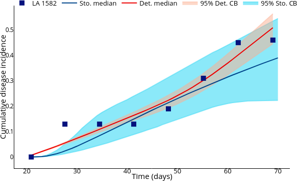
Data

  • Modelling

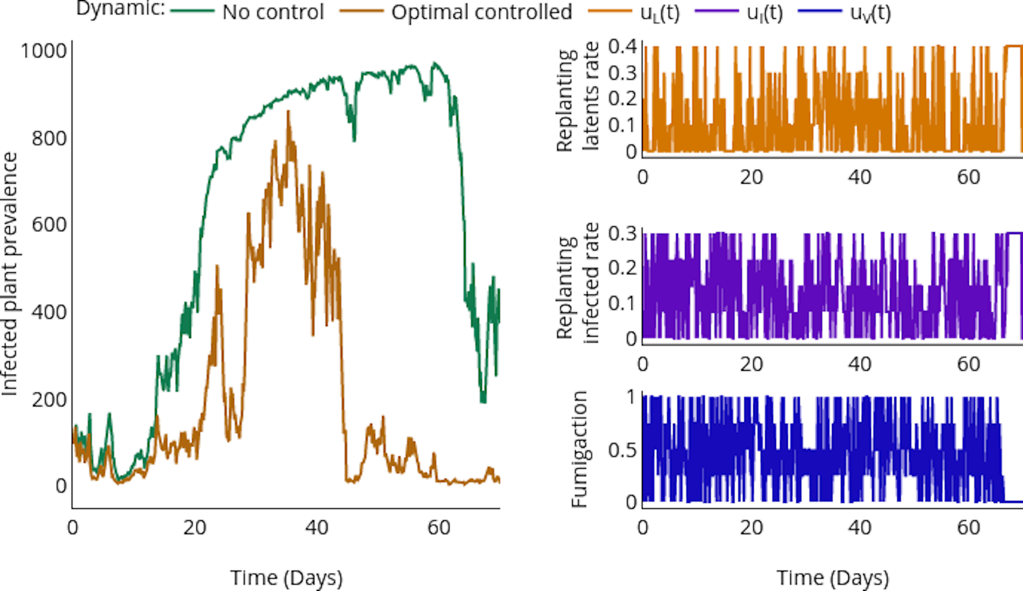
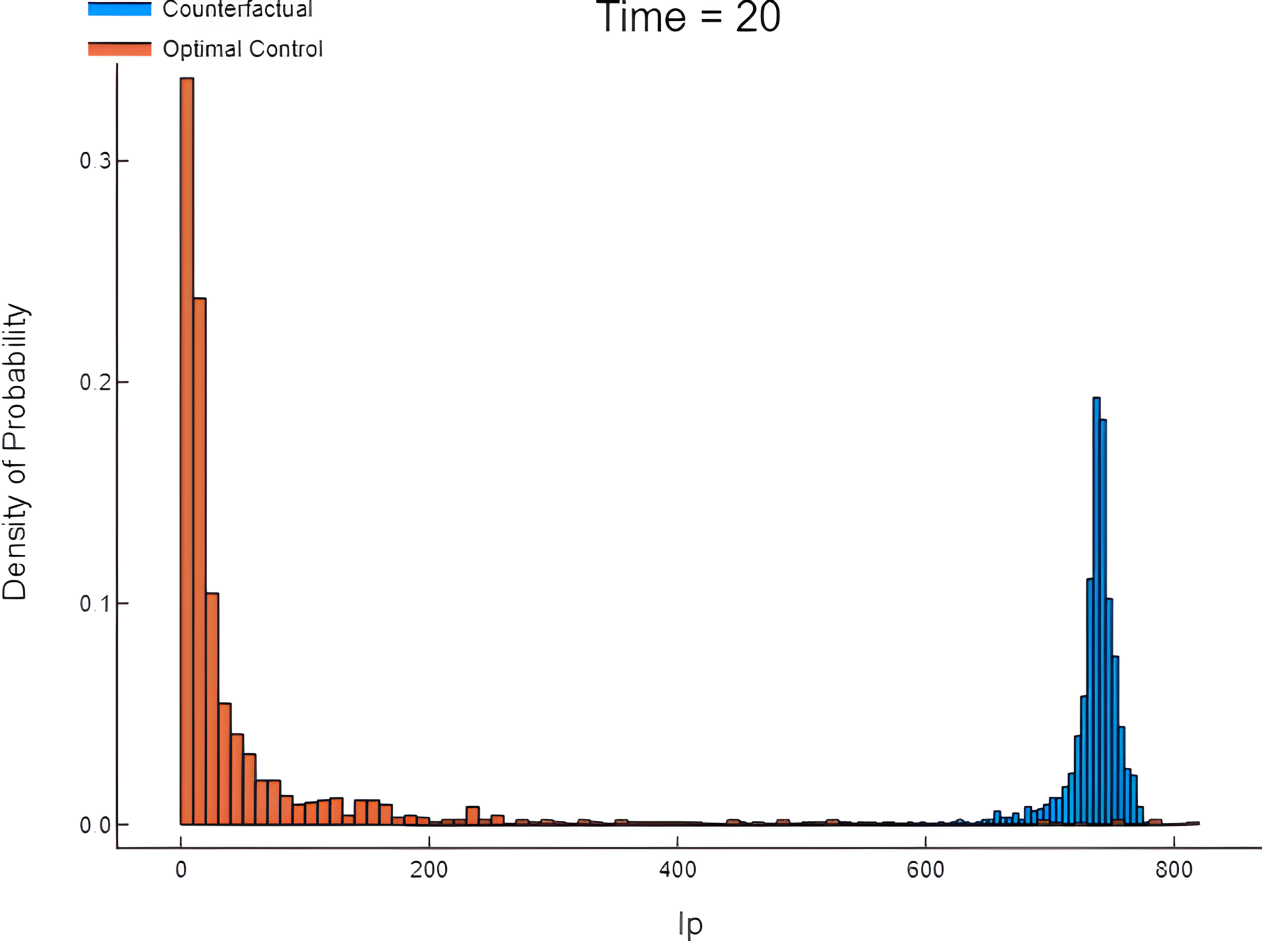
Control

To fix ideas:

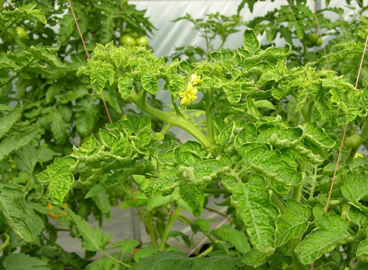
  • TYLCV Disease
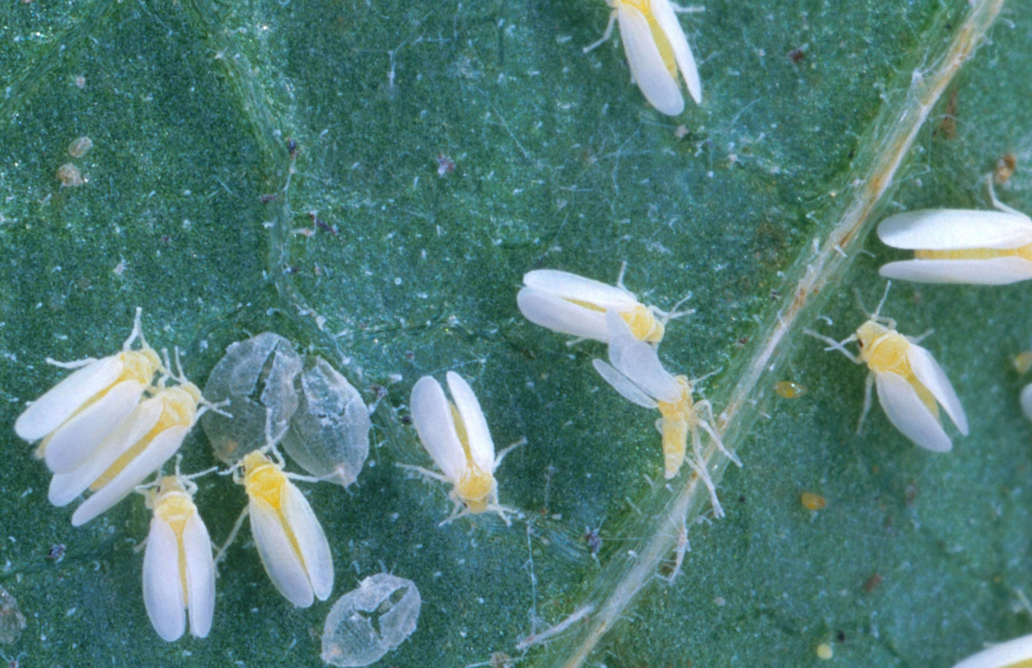
  • is spread by the insect whitefly (Bemisia tabaci)
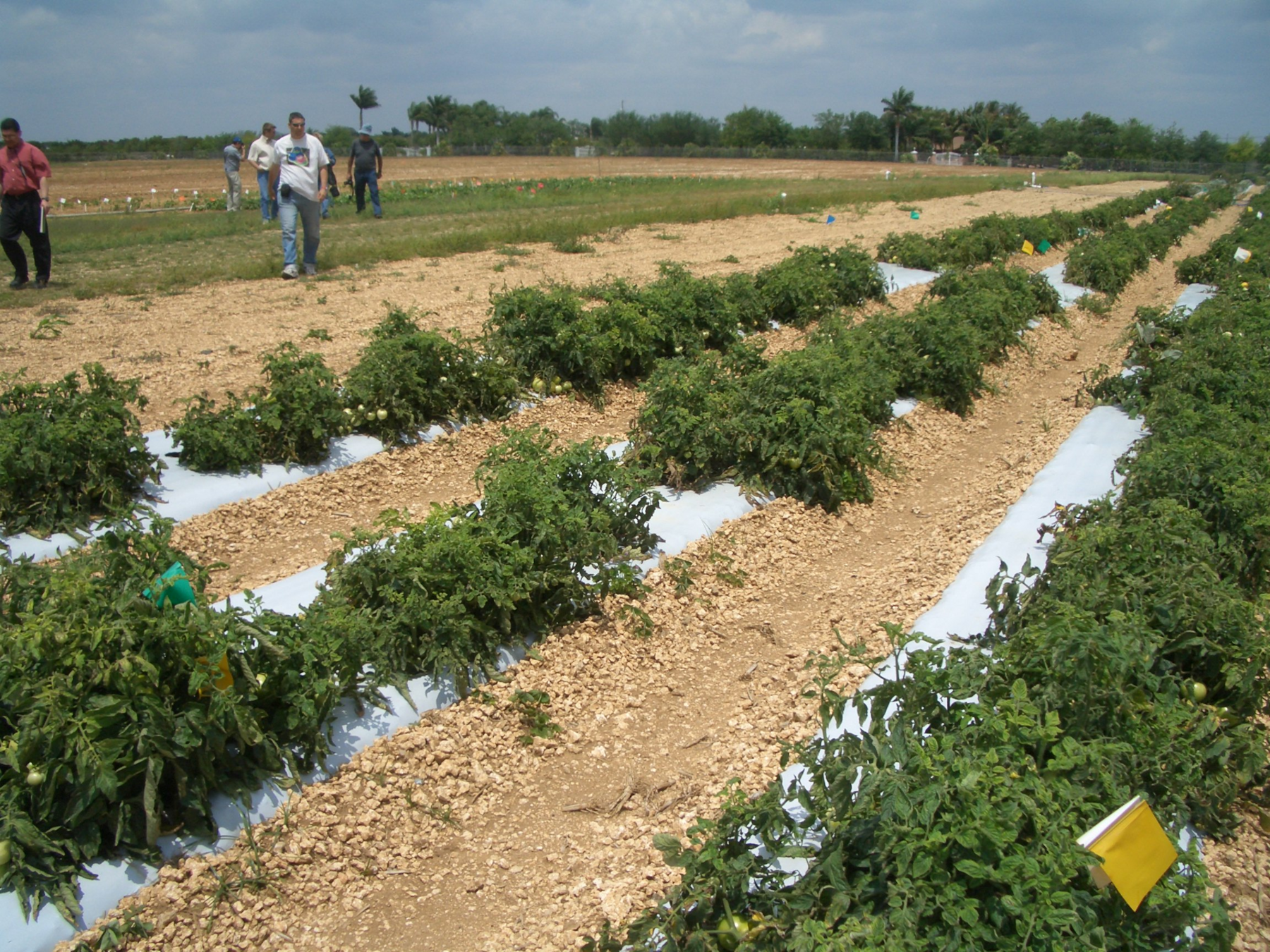
  • How to Manage TYLCV?
  • Replanting infected plants suffers random fluctuations due to is leading identification because a yellow plant is not necessarily infected.               

  • The protocol to manage infected plants suggests replanting neighbors. Then naturally, a farmer could randomly replant a healthy plant instead of a latent one.
  • Thus strategies like fumigation with insecticide suffer random fluctuationsin their efficiency.
Controls

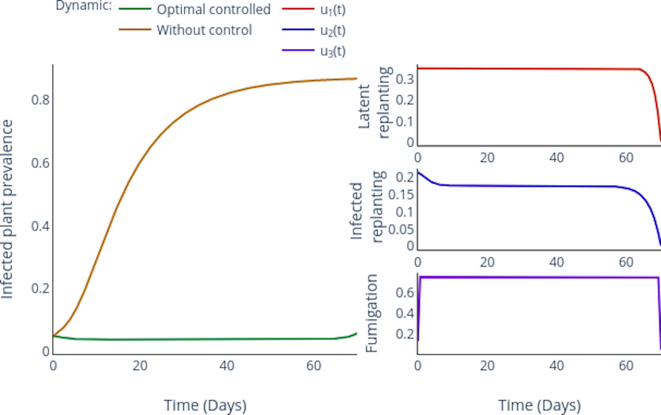
  • Replanting
  • Fumigation
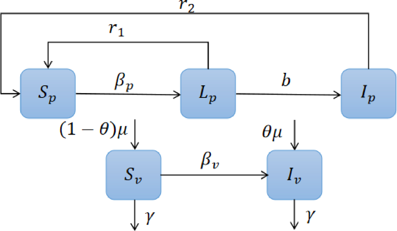
\begin{aligned} \dot{S_p} &= -\beta_p S_p I_v +\textcolor{blue}{r_1}L_p + \textcolor{blue}{r_2} I_p,\\ \dot{L_p} &= \beta_p S_p I_v -(b +\textcolor{blue}{r_1}) L_p,\\ \dot{I_p} &= b L_p - \textcolor{blue}{r_2} I_p,\\ \dot{S_v} &= -\beta_v S_v I_p - (\gamma +\textcolor{orange}{ \gamma_f}) S_v +(1-\theta)\mu,\\ \dot{I_v} &= \beta_v S_v I_p -(\gamma+\textcolor{orange}{\gamma_f}) I_v +\theta\mu. \end{aligned}
\begin{aligned} & \min_{\bar{u}(\cdot)\in \mathcal{U}_{x_0}[t_0,T]}J(u) \\ \text{Subject to} & \\ \dot{S_p} &= - \beta_p S_p I_v + \textcolor{blue}{(r_1 +u_1)} L_p + \textcolor{blue}{(r_2 + u_2)} I_p, \\ \dot{L_p} &= \beta_p S_p I_v -(b + \textcolor{blue}{(r_1 + u_1))} L_p, \\ \dot{I_p} &= b L_p - \textcolor{blue}{(r_2 + u_2)} I_p, \\ \dot{S_v} &= - \beta_v S_v I_p - (\gamma+ \textcolor{orange}{(\gamma_f + u_3)} ) S_v + (1-\theta)\mu, \\ \dot{I_v} &= \beta_v S_v I_p - (\gamma + \textcolor{orange}{(\gamma_f + u_3)}) I_v + \theta\mu, \\ &S_p(0) = S_{p_0}, L_p(0) = L_{p_0}, I_p(0) = I_{p_0}, \\ &S_v(0) = S_{v_0}, I_v(0) = I_{v_0}, u_i(t) \in [0, u_i ^ {max}]. \end{aligned}
\begin{aligned} J(u) &= \int_{0}^T \Big[A_1 I_p(t) + A_2 L_p(t) + A_3 I_v(t) + \sum^3_{i=1}c_i u_i(t)^2 \Big] dt, \end{aligned}

Enhancing parameter calibration through noise

\begin{aligned} \frac{d}{dt}x(t) = f(t,x(t)) & \rightsquigarrow dx(t) = f(t,x(t))dt + g(t,x(t))dB(t) \\ \alpha & \rightsquigarrow \alpha + P(x(t))\frac{dB(t)}{dt} \end{aligned}
\begin{aligned} \frac{dS_p}{dt} &= -\beta_p S_p \frac{I_v}{N_v} + \textcolor{blue}{r_1} L_p + \textcolor{blue}{r_2} I_p,\\ \frac{dL_p}{dt} &= \beta_p S_p \frac{I_v}{N_v} - (b + \textcolor{blue}{r_1}) L_p,\\ \frac{dI_p}{dt} &= b L_p - \textcolor{blue}{r_2} I_p,\\ \frac{dS_v}{dt} &= -\beta_v S_v \frac{I_p}{N_p} - (\gamma + \textcolor{orange}{\gamma_f}) S_v + (1-\theta)\mu,\\ \frac{dI_v}{dt} &= \beta_v S_v \frac{I_p}{N_p} - (\gamma + \textcolor{orange}{\gamma_f}) I_v +\theta\mu,\\ \end{aligned}
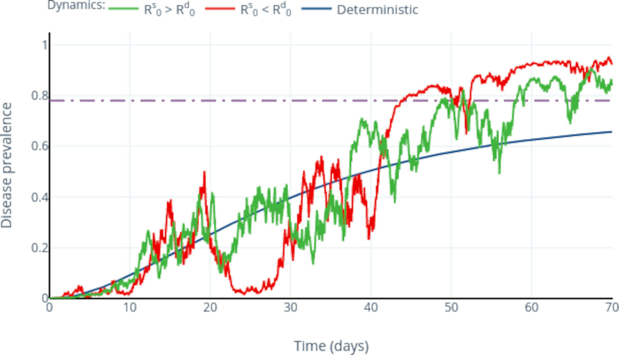
\begin{aligned} r_1 dt \rightsquigarrow r_1 dt + \sigma_L\frac{S_p}{N_p}dB_p(t), \\ r_2 dt \rightsquigarrow r_2 dt + \sigma_I\frac{S_p}{N_p} dB_p(t), \\ \gamma_f dt \rightsquigarrow \gamma_f dt + \sigma_v dB_v(t). \end{aligned}
\begin{aligned} d S_p &= \left( -\beta_p S_p \frac{I_v}{N_v} + \textcolor{blue}{r_1} L_p + \textcolor{blue}{r_2} I_p \right)dt + \textcolor{blue}{\frac{S_p(\sigma_L L_p + \sigma_I I_p)}{N_p}} dB_p(t), \\ dL_p &= \left( \beta_p S_p \frac{I_v}{N_v} - (b + \textcolor{blue}{r_1}) L_p \right) dt - \textcolor{blue}{\sigma_L \frac{S_p L_p}{N_p}} dB_p(t), \\ d I_p &= \left( b L_p - \textcolor{blue}{r_2} I_p \right) dt - \textcolor{blue}{\sigma_I \frac{S_pI_p}{N_p}} dB_p(t), \\ dS_v &= \left( -\beta_v S_v \frac{I_p}{N_p} - (\gamma + \textcolor{orange}{\gamma_f}) S_v + (1-\theta) \mu \right)dt - \textcolor{orange}{\sigma_v S_v} dB_v(t), \\ d I_v &= \left( \beta_v S_v \frac{I_p}{N_p} - (\gamma + \textcolor{orange}{\gamma_f}) I_v + \theta \mu \right) dt - \textcolor{orange}{\sigma_v I_v} dB_v(t). \end{aligned}
const { data: unknownAssetsBalances } = useQueriesData(
    unknownAssetsIds.map((id) => ({
      ...queries.assets.balances.addressToken(addressHash, id),
      enabled: unknownAssetsIds.length > 0
    }))
  )

  let tokensWithBalanceAndMetadata = flatMap(tokenBalances, (t) => {
    const metadata = find(fungibleTokens, { id: t.id })

    return metadata ? [{ ...t, ...metadata, balance: BigInt(t.balance), lockedBalance: BigInt(t.lockedBalance) }] : []
  })

  tokensWithBalanceAndMetadata = sortBy(tokensWithBalanceAndMetadata, [
    (t) => !t.verified,
    (t) => !t.name,
    (t) => t.name.toLowerCase(),
    'id'
  ])
\begin{aligned} dx(t) &= f(t, x(t), \textcolor{orange}{u(t)})dt + g(t, x(t), u(t)) dW(t),\\ x(0) &= x_0 \in \mathbb{R}^n, \\ \\ J(u(\cdot)) &= \mathbb{E} \left\{ \int^T_0 c(t,x(t),u(t)) dt + h(x(T))\right\}. \end{aligned}
\begin{aligned} &J(\bar{\pi}) = \inf_{\pi \in\, \mathcal{U}[0,T]} J(\pi)\\ \text{Suject to}&\\ dx(t) &= f(t, x(t), u(t))dt + g(t, x(t), u(t)) dW(t),\\ x(0) &= x_0 \in \mathbb{R}^n, \end{aligned}
\begin{aligned} \forall t & \in[0,T], \ x, \ \hat{x} \in \mathbb{R}^n, \ u \in U, \\ &|\varphi(t,x,u) - \varphi(t, \hat{x},u)|\leq L|x-\hat{x}|, \end{aligned}
\begin{aligned} f:[0,T] \times \mathbb{R} ^ n \times U &\to \mathbb{R}^n, \\ g:[0,T] \times\mathbb{R} ^ n \times U &\to \mathbb{R}^{n\times m}, \\ c:[0,T] \times\mathbb{R} ^ n \times U &\to \mathbb{R}, \\ h:\mathbb{R}^n \to \mathbb{R}& \end{aligned}
\begin{aligned} (s,y) \in [0,T) &\times \mathbb{R}^n, \\ V(s,y) &= \inf_{ u(\cdot) \in \mathcal{U} [s,T]} J(s, y; u(\cdot) ), \\ V(T,y) &= h(y), \qquad \forall y\in \mathbb{R}^n, \end{aligned}
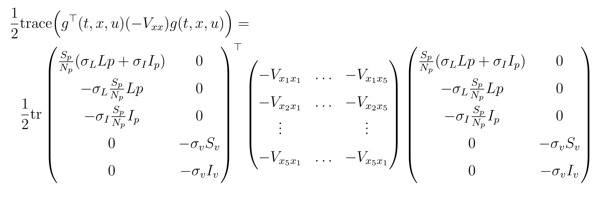
\begin{aligned} & -V_t + \sup_{u \in U} H_G (t ,x, u, -V_x, -V_{xx})=0, (t,x) \in [0,T)\times\mathbb{R}^n, \\ & V \Big|_{t=T} = h(x), \qquad x\in \mathbb{R} ^ n, \\ & H_G(t,x,u,p,P) = \langle p, f(t,x,u) \rangle - c(t,x,u) \\ &+\dfrac{1}{2} \mathtt{trace}\Big( g^\top(t,x,u)Pg(t,x,u)\Big) \\ & = H_{det}(t,u,x,p) +\dfrac{1}{2} \mathtt{trace}\Big( g^\top(t,x,u)Pg(t,x,u)\Big) \end{aligned}
\begin{aligned} \forall (t,u) & \in [0,T]\times U \\ &|\varphi(t,0,u)|\leq L \end{aligned}

OPC:

Value Function

HJB

\begin{aligned} dx(t) &= f(t, x(t), \textcolor{orange}{u(t)})dt + g(t, x(t), u(t)) dW(t),\\ x(0) &= x_0 \in \mathbb{R}^n, \\ J(u(\cdot)) &= \mathbb{E} \left\{ \int^T_0 c(t,x(t),u(t)) dt + h(x(T))\right\}. \end{aligned}
\begin{aligned} J(u) = \mathbb{E}\int_{0}^{T} & \Bigg[ A_1 I_p(t) + A_2 L_p(t) + A_3 I_v (t) \\ & + c_1 u ^ 2_1(t) + c_2 u ^ 2_2(t) + c_3 u ^ 2_3(t) \Bigg] dt, \end{aligned}
\begin{aligned} &\qquad\qquad\qquad\qquad\min_{u\in \mathcal{U}[0,T]} J(u) \\ &\qquad \text{subject to } \\ &dS_p = \left( -\beta_pS_p\frac{I_v}{N_v}+(r_1 +u_1) L_p + (r_2 + u_2)L_p \right)dt \\ &+ \frac{S_p}{N_p}\left( \sigma_L L_p+\sigma_I I_p \right)dB_p,\\ &dL_p = \left( \beta_pS_p\frac{I_v}{N_v}-(b+r_1 +u_1)L_p \right)dt -\sigma_L\frac{S_p}{N_p}L_pdB_p, \\ &dI_p = \left( b L_p - (r_2 + u_2) I_p \right)dt - \sigma_I\frac{S_p}{N_p}I_p dB_p, \\ &dS_v = \left( -\frac{\beta_v}{N_p}S_vI_p -(\gamma +\gamma_f+ u_3) S_v + (1-\theta)\mu\right)dt -\sigma_v S_vdB_v, \\ &dI_v = \left( \frac{\beta_v}{N_p}S_vI_p - (\gamma +\gamma_f+u_3) I_v +\theta \mu \right) dt - \sigma_v S_v dB_v. \end{aligned}
\begin{aligned} V(s,x) = \inf_{u(\cdot) \in \mathcal {U}[s,T]} &\mathbb{E} \Bigg\{ \int_{s}^{T} \Big[ A_1 I_p(t) + A_2 L_p(t) + A_3 I_v (t) \\ & + c_1 u ^ 2_1(t) + c_2 u ^ 2_2(t) + c_3 u ^ 2_3(t) \Big] dt \Bigg\} \end{aligned}
\begin{aligned} &-V_t + \sup_{u \in U} H_G(t, x, u, -V_x, -V_{xx})=0 \end{aligned}
\begin{aligned} H_G(t,x,u,p,P) &= \langle p, f(t,x,u) \rangle - c(t,x,u) \\ &+\dfrac{1}{2} \mathtt{trace}\Big( g^\top(t,x,u)Pg(t,x,u)\Big) \end{aligned}
\begin{aligned} H_{det} &(t,u,x,-V_x) = A_1I_v+A_2L_p+A_3I_v +\sum_{i=1}^{3}c_iu_i^2\\ &-V_{x_1}(-\beta_p S_p I_v +(r_1 +u_1)L_p + (r_2 + u_2) I_p)\\ & -V_{x_2}(\beta_p S_p I_v-(b +r_1 + u_1)L_p)\\ &-{V_{x_3}}(b L_p - (r_2 + u_2) I_p)\\ &-V_{x_4}(-\beta_v S_v I_p - (\gamma+\gamma_f+u_3) S_v +(1-\theta)\mu)\\ &-V_{x_5}(\beta_v S_v I_p -(\gamma+\gamma_f+u_3) I_v+\theta\mu). \end{aligned}
HJB (Dynamic Programming)
  • Course of dimensionality
\approx \ \mathtt{HJB}
HJB (Neuro-Dynamic Programming)

Bertsekas, Dimitri P.

Abstract dynamic programming.

Athena Scientific, Belmont, MA, 2013. viii+248 pp.

ISBN:978-1-886529-42-7

ISBN:1-886529-42-6

Bertsekas, Dimitri P.

Rollout, policy iteration, and distributed reinforcement learning.

Revised and updated second printing

Athena Sci. Optim. Comput. Ser.

Athena Scientific, Belmont, MA, [2020], ©2020. xiii+483 pp.

ISBN:978-1-886529-07-6

Reinforcement learning and optimal control

Bertsekas, Dimitri P.

Athena Sci. Optim. Comput. Ser.

Athena Scientific, Belmont, MA, 2019, xiv+373 pp.

ISBN: 978-1-886529-39-7
Gracias

1.Salcedo-Varela, G. & Diaz-Infante, S. Threshold behaviour of a stochastic vector plant model for Tomato Yellow Curl Leaves disease: a study based on mathematical analysis and simulation. Int J Comput Math 1–0 (2022) doi:10.1080/00207160.2022.2152680.


2. Salcedo‐Varela, G. A., Peñuñuri, F., González‐Sánchez, D. & Díaz‐Infante, S. Synchronizing lockdown and vaccination policies for COVID‐19: An optimal control approach based on piecewise constant strategies. Optim. Control Appl. Methods (2023) doi:10.1002/oca.3032.


3.Diaz-Infante, S., Gonzalez-Sanchez, D. & Salcedo-Varela, G. Handbook of Visual, Experimental and Computational Mathematics, Bridges through Data. 1–19 (2023) doi:10.1007/978-3-030-93954-0_37-1.


https://slides.com/sauldiazinfantevelasco/slides_red_mex_bio_mat

Slide RedMexBio

By Saul Diaz Infante Velasco

Slide RedMexBio

Talk for the First Evet for the RedMexBioMat

  • 42