


Dr. Sergey Kosov
University Lecturer and Entrepreneur
Dr. Sergey Kosov
Assumes that the PDF of random variables have normal (Gaussian) distribution
$$\mathcal{N}(\vec{y};~\vec{\mu}, \Sigma) = \frac{1}{(2\pi)^{m/2}} \frac{1}{|\Sigma|^{1/2}}\exp{\left(-\frac{1}{2}(y-\mu)^\top\Sigma^{-1}(y-\mu)\right)}$$
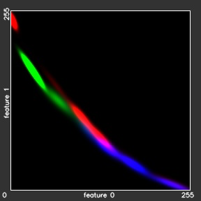
+ Models the conditional dependencies of all features \(f_i(y)\) via covariance matrix \(\Sigma\)
- Can't model complex non-Gaussian distributions
Assumes that the PDF of random variables can be modeled by a linear combination of multiple Gaussians $$\sum_i\mathcal{N}_i(\vec{y};~\vec{\mu}_i, \Sigma_i)$$
+ Can model complex non-Gaussian distributions
+ One of the most accurate methods among generative approaches
The average value of a random function \(f(x)\) under a probability distribution \(p(x)\) is called the expectation of \(f(x)\) and denoted through \(E[f(x)]\):
$$E[f(x)]=\sum p(x)f(x)$$
$$E[f(x)]=\int\limits^{\infty}_{-\infty}p(x)f(x)dx$$
The variance of a random function \(f(x)\) is the expected value of the squared deviation from the mean of \(f(x)\),
here mean \(\mu=E[f(x)]\)
$$Var[f(x)]=E[(f(x)-E[f(x)])^2]$$
$$E[(f(x)-E[f(x)])^2]=E[f(x)^2]-E[f(x)]^2$$
If a random variable \(y\) has normal distribution:
We therefore consider a superposition of \(G\) Gaussian densities of the form:
$$\mathcal{P}(\vec{y}) = \sum^{G}_{k=1}\omega_k\mathcal{N}_k(\vec{y};~\vec{\mu}_k,\Sigma_k)$$
which is called a mixture of Gaussians.
Each Gaussian density \(\mathcal{N}_k(\vec{y};~\vec{\mu}_k,\Sigma_k)\) is called a mixture component of the mixture and has its own mean \(\vec{\mu}_k\) and covariance \(\Sigma_k\)
The weights \(\omega_k\) are called mixture coefficients
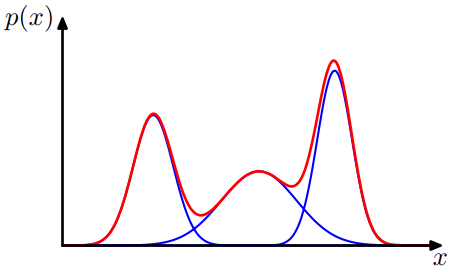
The Gaussian mixture distribution in 1D formed by 3 Gaussians
$$\mathcal{P}(y)=\omega_1\mathcal{N}_1+\omega_2\mathcal{N}_2 + \omega_3\mathcal{N}_3$$
Source: Christopher M. Bishop's textbook “Pattern Recognition & Machine Learning”
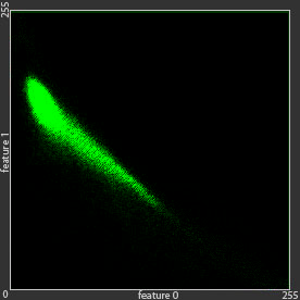
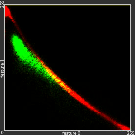
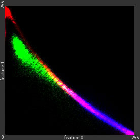
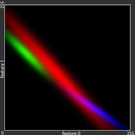
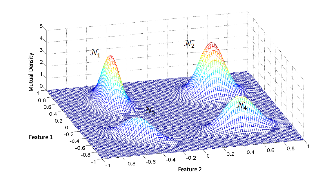
The Gaussian mixture distribution in 2D formed by 4 Gaussians
$$\mathcal{P}(\vec{y})=\omega_1\mathcal{N}_1+\omega_2\mathcal{N}_2 + \omega_3\mathcal{N}_3+\omega_4\mathcal{N}_4$$
If we integrate both sides of equation
\(\mathcal{P}(\vec{y}) = \sum^{G}_{k=1}\omega_k\mathcal{N}_k(\vec{y};~\vec{\mu}_k,\Sigma_k)\) with respect to \(\vec{y}\), and note that both \(\mathcal{P}(\vec{y})\) and the individual Gaussian components are normalised, we obtain \(\sum^{G}_{k=1}\omega_k=1\).
Also, given that \(\mathcal{N}_k(\vec{y};~\vec{\mu}_k, \Sigma_k)\ge0\), a sufficient condition for the requirement \(\mathcal{P}(\vec{y})\ge0\) is that \(\omega_k\ge0, \forall k \in [1; G]\). Combining this with the condition above we obtain \(0\le\omega_k\le1\).
We therefore see that the mixture coefficients satisfy the requirements to be probabilities, and so, could be considered as as the prior probabilities of picking the k-th component.
The densities \(\mathcal{N}_k(\vec{y};~\vec{\mu}_k, \Sigma_k)\), in its turn, could be considered as the probabilities of \(\vec{y}\) conditioned on \(k\): \(p(\vec{y}~|~k)\).
From Bayes' theorem we can write:
$$p(\vec{y}~|~k)\propto p(\vec{y})\cdot p(\vec{y}~|~k) = \omega_k\mathcal{N}_k(\vec{y};~\vec{\mu}_k,\Sigma_k)$$
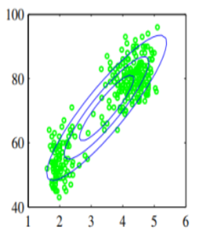
The green dot are an example of given data that cannot be modelled using single Gaussian distribution, because it has two clusters or summits.
To model green dots distributions, we can use linear combination of Gaussian distributions , which is much better than single Gaussian distribution.
is the estimation of mixture coefficients \(\omega_k\) and parameters of the mixture components \(\vec{\mu}_k\), \(\Sigma_k\) from training dataset
Split the training samples into some number \(K\) of clusters using for example a non-probabilistic technique called the K-means algorithm.
is the estimation of mixture coefficients \(\omega_k\) and parameters of the mixture components \(\vec{\mu}_k\), \(\Sigma_k\) from training dataset
alternates between performing an expectation (E) step and a maximization (M) step:
Expectation maximization algorithm takes several iterations in order to reach (approximate) convergence and each cycle requires heavy computation.
It requires the simultaneous storage and processing of all the training samples and the prior definition of the number \(G\) of Gaussians in the mixture model.
is the estimation of mixture coefficients \(\omega_k\) and parameters of the mixture components \(\vec{\mu}_k\), \(\Sigma_k\) from training dataset
is used to overcome the limitations of the expectation maximization algorithm.
Two assumptions on training sample points
Sequential methods allow data points to be processed one at a time and then discarded and are important for online applications, and also where large data sets are involved so that batch processing of all data points at once is infeasible.
Arthur P. Dempster, Nan M. Laird, and Donald B. Rubin. “Maximum likelihood from incomplete data via the EM algorithm.” In: Journal of the Royal Statistical Society: Series B 39.1 (1977), pp. 1–38
OpenCV library: cv::ml::EM Class Reference
Sergey G. Kosov, Franz Rottensteiner and Christian Heipke: "Sequential Gaussian Mixture Models for Two-Level Conditional Random Fields", In: Proceedings of the 35th German Conference on Pattern Recognition (GCPR). Vol. 8142. Lecture Notes in Computer Science. Springer, 2013, pp. 153–163
DGM library: DGM::CTrainNodeGMM Class Reference
Multivariate Gaussian Implementation: CKDGauss.h CKDGauss.cpp
Estimation of the GMMparameters (learning): CTrainNodeGMM.h CTrainNodeGMM.cpp
By Dr. Sergey Kosov
This lecture is intended to familiarise students with the concepts of mixture distributions and their estimation. It presents both the difficulties that arise and concrete approaches to solving them.


