
Lecture 3: Gradient Descent Methods
Intro to Machine Learning

- That formula is not well-defined 👉
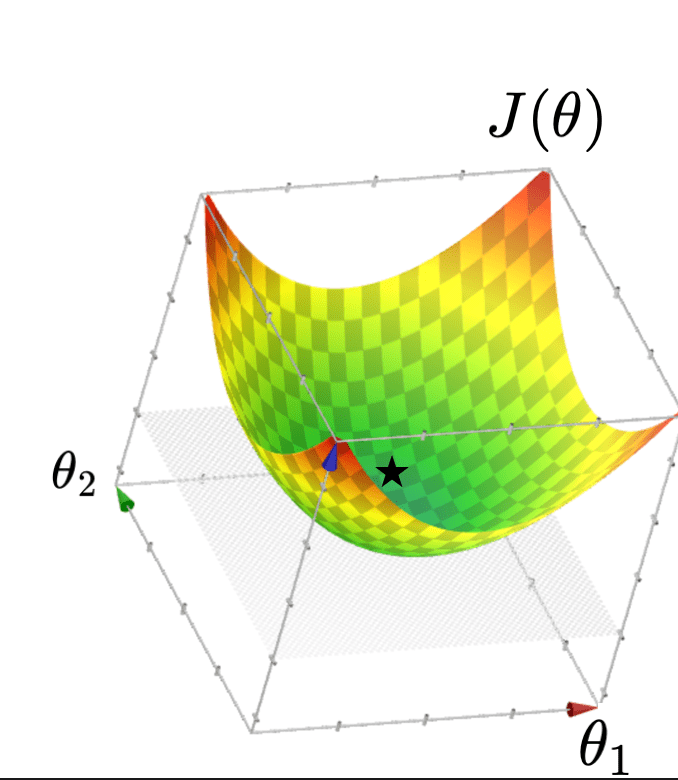
Typically, \(X\) is full column rank
- \(\theta^*=\left({X}^{\top} {X}\right)^{-1} {X}^{\top} {Y}\)
- \(J(\theta)\) "curves up" everywhere
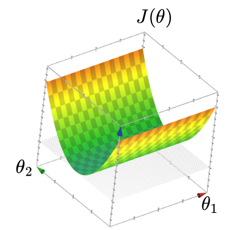
When \(X\) is not full column rank
- \(J(\theta)\) has a "flat" bottom
- Infinitely many optimal hyperplanes
- unique optimal hyperplane
\(\theta^*\) can be costly to compute (lab2 Q2.8)
No way yet to get any \(\theta^*\)
\(\theta^*\) numerically sensitive
Recall:
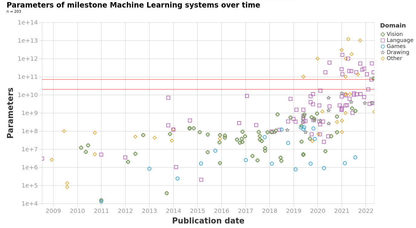
https://epoch.ai/blog/machine-learning-model-sizes-and-the-parameter-gap
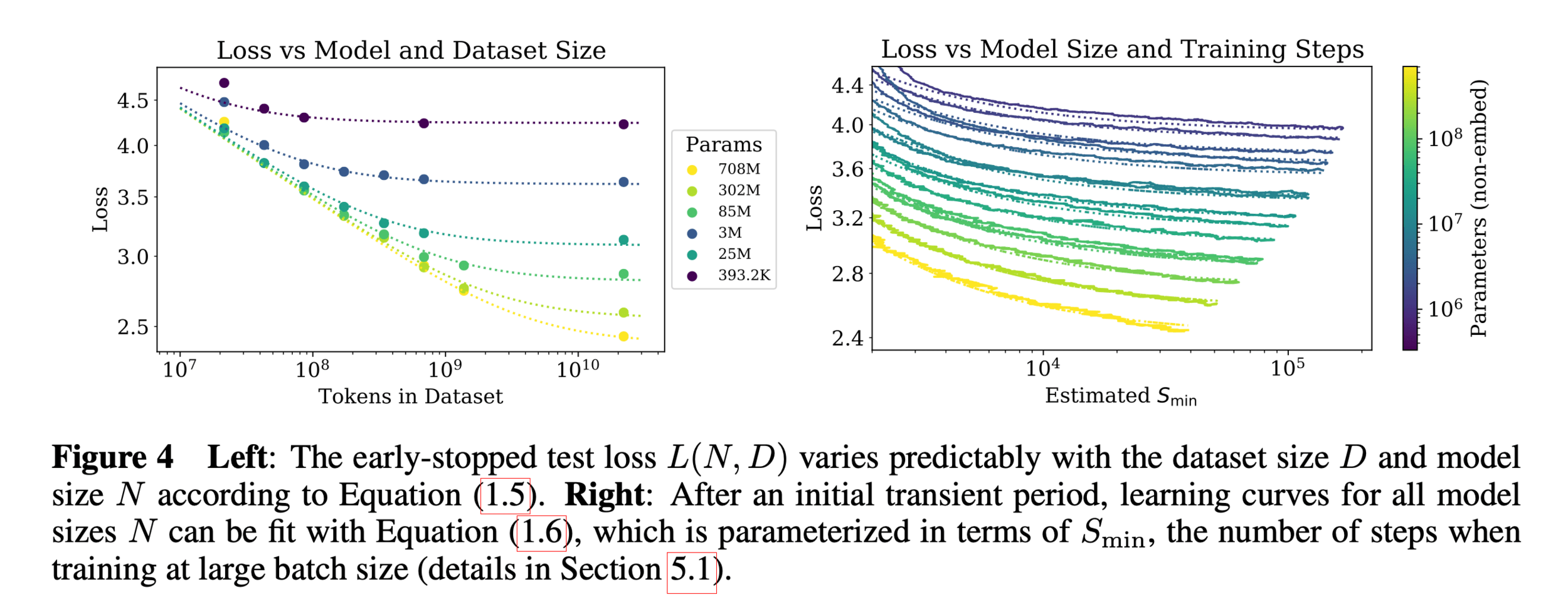
https://arxiv.org/pdf/2001.08361
In the real world,
- the number of parameters is huge
- the number of training data points is huge
- hypothesis class is typically highly nonlinear
- loss function is rarely as simple as squared error
Need a more efficient and general algorithm to train our ML system
⇒ gradient descent methods
Outline
-
Gradient descent (GD)
- The gradient vector
- GD algorithm
- Gradient descent properties
- Stochastic gradient descent (SGD)
For \(f: \mathbb{R}^m \rightarrow \mathbb{R}\), its gradient \(\nabla f: \mathbb{R}^m \rightarrow \mathbb{R}^m\) is defined at the point \(p=\left(x_1, \ldots, x_m\right)\) as:
\nabla f(p)=\left[\begin{array}{c}
\frac{\partial f}{\partial x_1}(p) \\
\vdots \\
\frac{\partial f}{\partial x_m}(p)
\end{array}\right]
The gradient may not always exist or be well-behaved.
Today, we have nice gradients unless otherwise specified.
- The gradient generalizes the concept of a derivative to multiple dimensions.
- By construction, the gradient has the same dimension as the function's input.
\nabla f(p)=\left[\begin{array}{c}
\frac{\partial f}{\partial x_1}(p) \\
\vdots \\
\frac{\partial f}{\partial x_m}(p)
\end{array}\right]
3. The gradient can be symbolic or numerical.
f(x, y, z) = x^2 + y^3 + z
e.g.,
its symbolic gradient:
just like a derivative can be a function or a number.
evaluating the symbolic gradient at a point gives a numerical gradient:
\nabla f(x, y, z) = \begin{bmatrix}
2x \\
3y^2 \\
1
\end{bmatrix}
\nabla f(3, 2, 1) = \nabla f(x,y,z)\Big|_{(x,y,z)=(3,2,1)} = \begin{bmatrix}6\\12\\1\end{bmatrix}
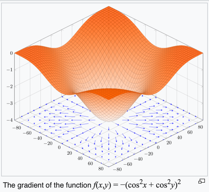
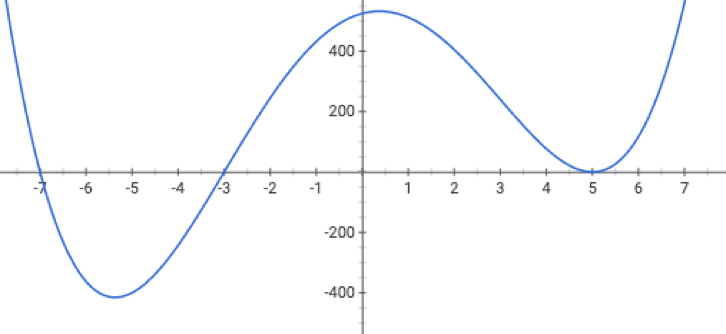
4. The gradient points in the direction of the (steepest) increase in the function value.
\(\frac{d}{dx} \cos(x) \bigg|_{x = -4} = -\sin(-4) \approx -0.7568\)
\(\frac{d}{dx} \cos(x) \bigg|_{x = 5} = -\sin(5) \approx 0.9589\)
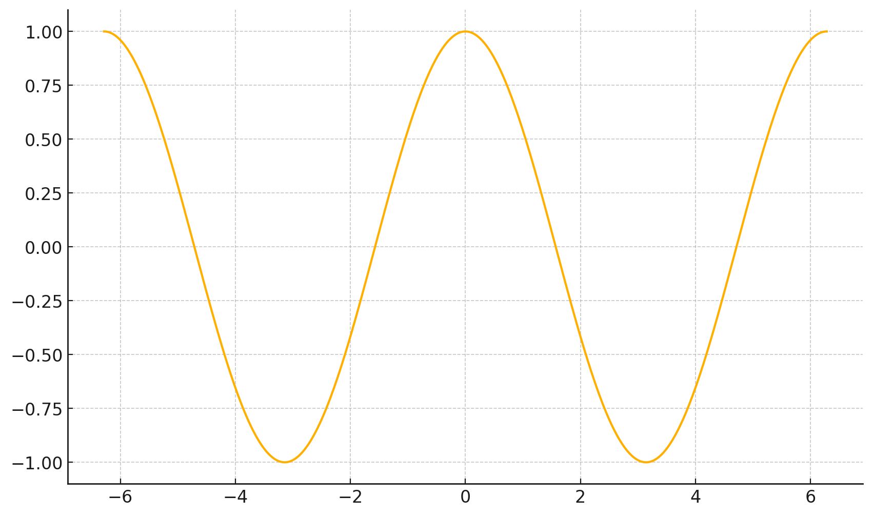
f(x)=\cos(x)
x
5. For \(f\) defined on all of \(\mathbb{R}^m\), the gradient at a minimizer is necessarily zero.
f(x)=\cos(x)
x
For \(f: \mathbb{R}^m \rightarrow \mathbb{R}\), its gradient \(\nabla f: \mathbb{R}^m \rightarrow \mathbb{R}^m\) is defined at the point \(p=\left(x_1, \ldots, x_m\right)\) as:
\nabla f(p)=\left[\begin{array}{c}
\frac{\partial f}{\partial x_1}(p) \\
\vdots \\
\frac{\partial f}{\partial x_m}(p)
\end{array}\right]
The gradient may not always exist or be well-behaved.
In our context, \(J\) plays the role of \(f\), \(\theta\) plays \(p.\)
- The gradient generalizes the concept of a derivative to multiple dimensions.
- By construction, the gradient has the same dimension as the function's input.
- The gradient can be symbolic or numerical.
- The gradient points in the direction of the (steepest) increase in the function value.
- For \(f\) defined on all of \(\mathbb{R}^m\), the gradient at a minimizer is necessarily zero.
Outline
-
Gradient descent (GD)
- The gradient vector
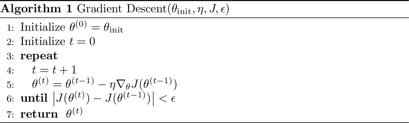
- GD algorithm
- Gradient descent properties
- Stochastic gradient descent (SGD)
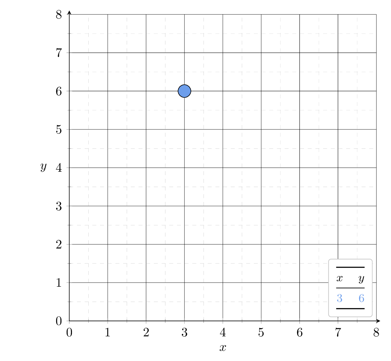
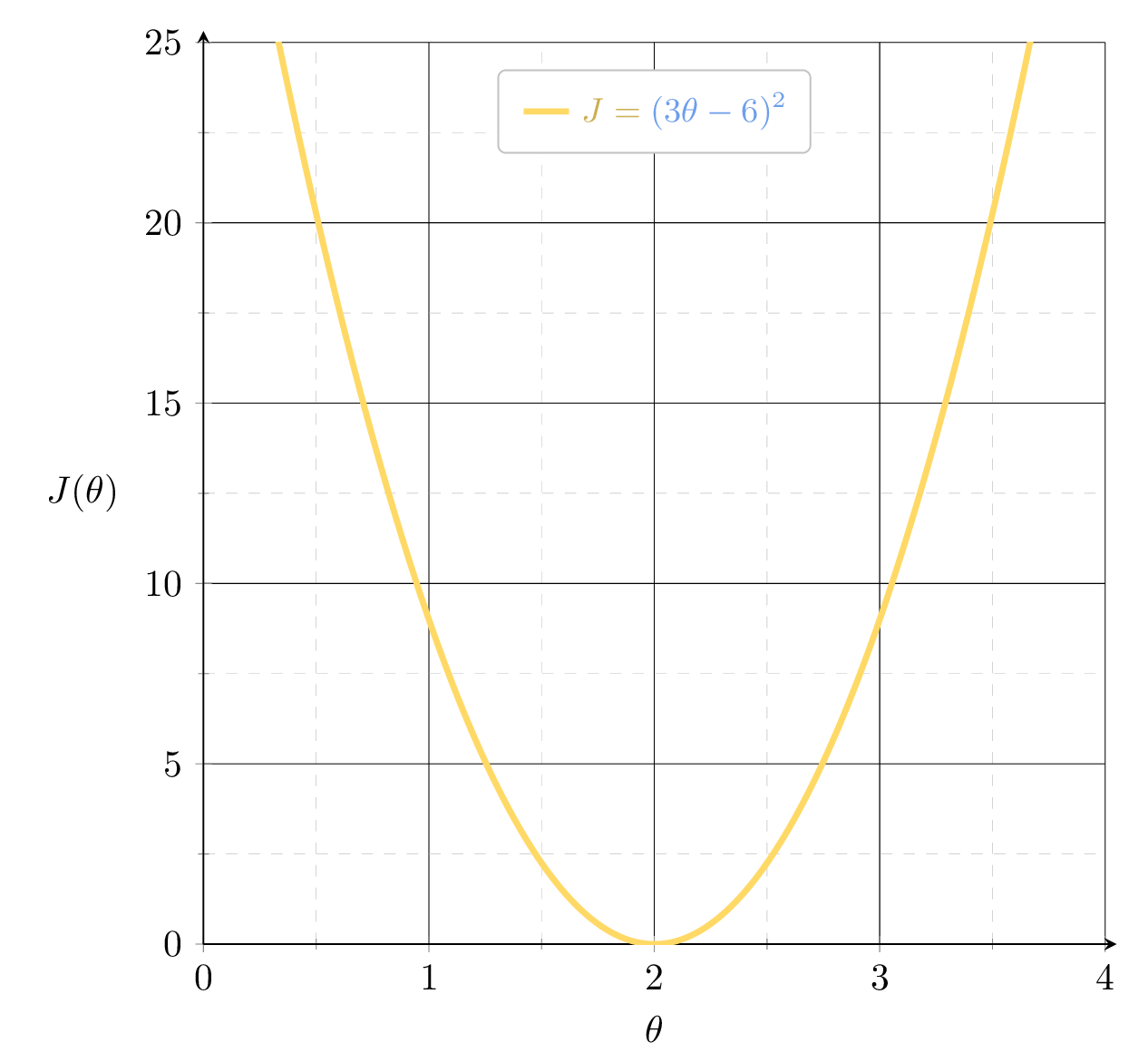
Example 1: fit a line (no offset) to minimize MSE
Suppose we fit \(h= 1.5x\)
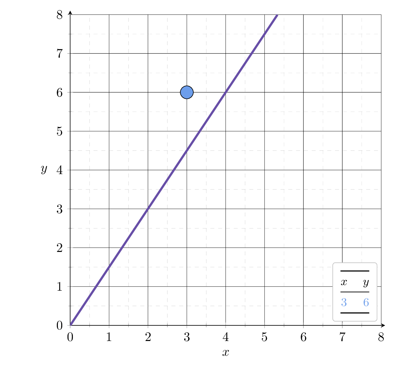
1.5
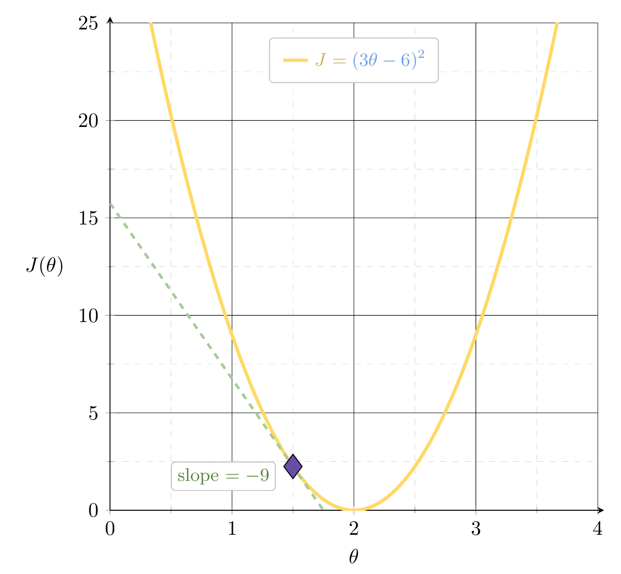
MSE could get better, by leveraging the gradient
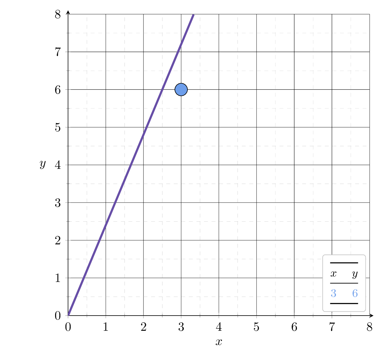
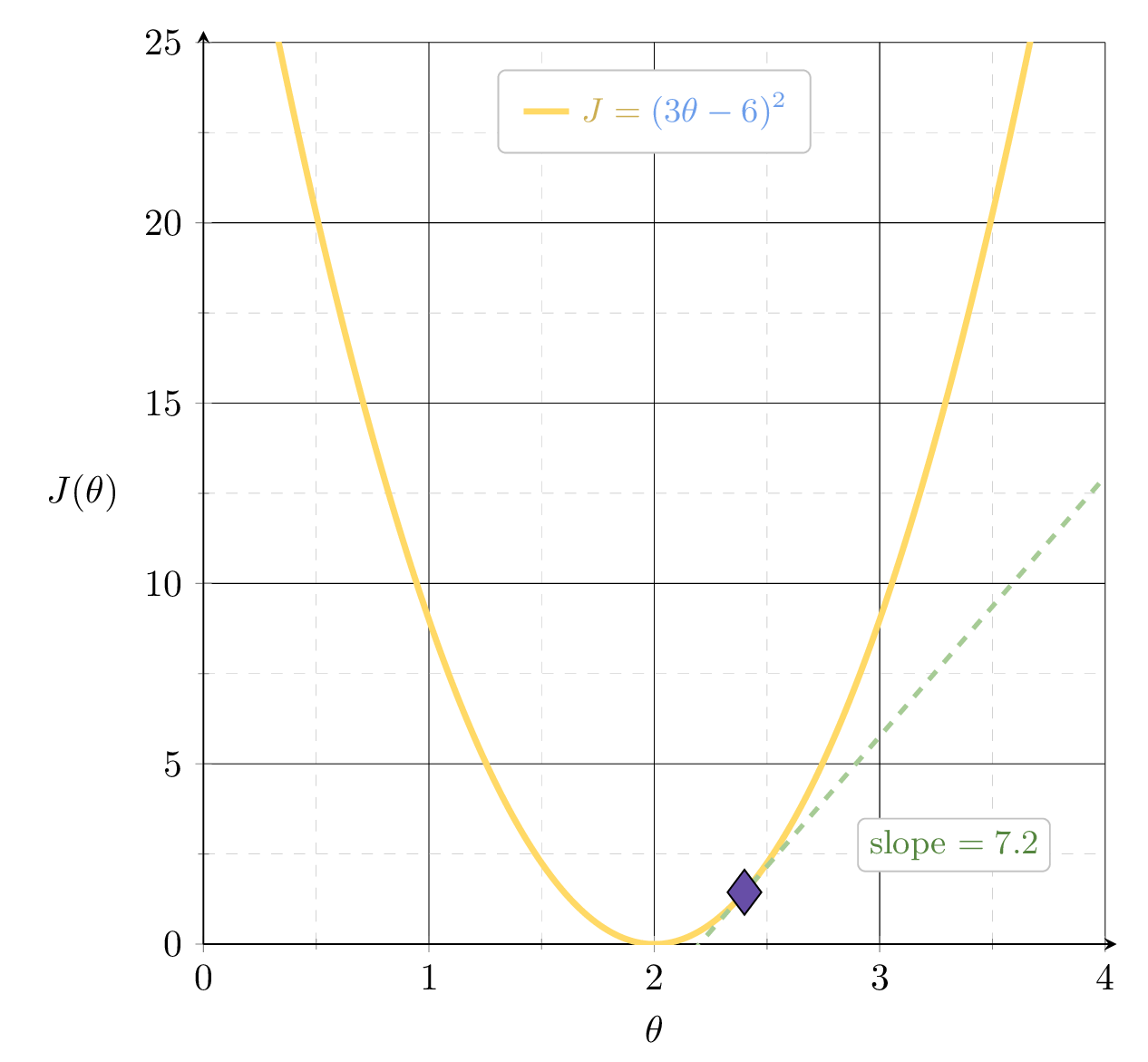
MSE could get better, by leveraging the gradient
Suppose we fit \(h= 2.4x\)
2.4
Example 1: fit a line (no offset) to minimize MSE
hyperparameters
initial guess of parameters
learning rate
precision
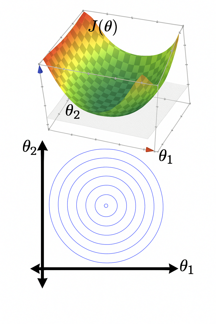
level set,
contour plot

iteration counter
objective improvement is nearly zero.
Other possible stopping criterion for line 6:
- Small parameter change: \( \|\theta^{(t)} - \theta^{(t-1)}\| < \epsilon \), or
- Small gradient norm: \( \|\nabla_{\theta} J(\theta^{(t-1)})\| < \epsilon \)
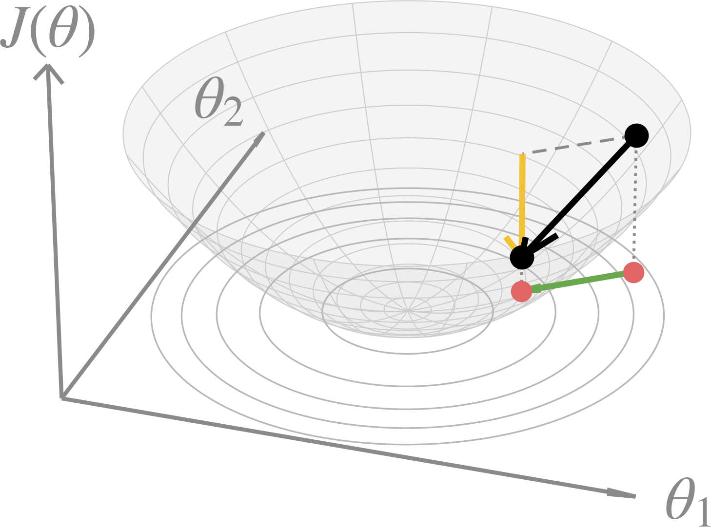
What does this 2d vector represent? anything in the pseudocode?
What does this 3d vector represent? anything in the pseudocode?
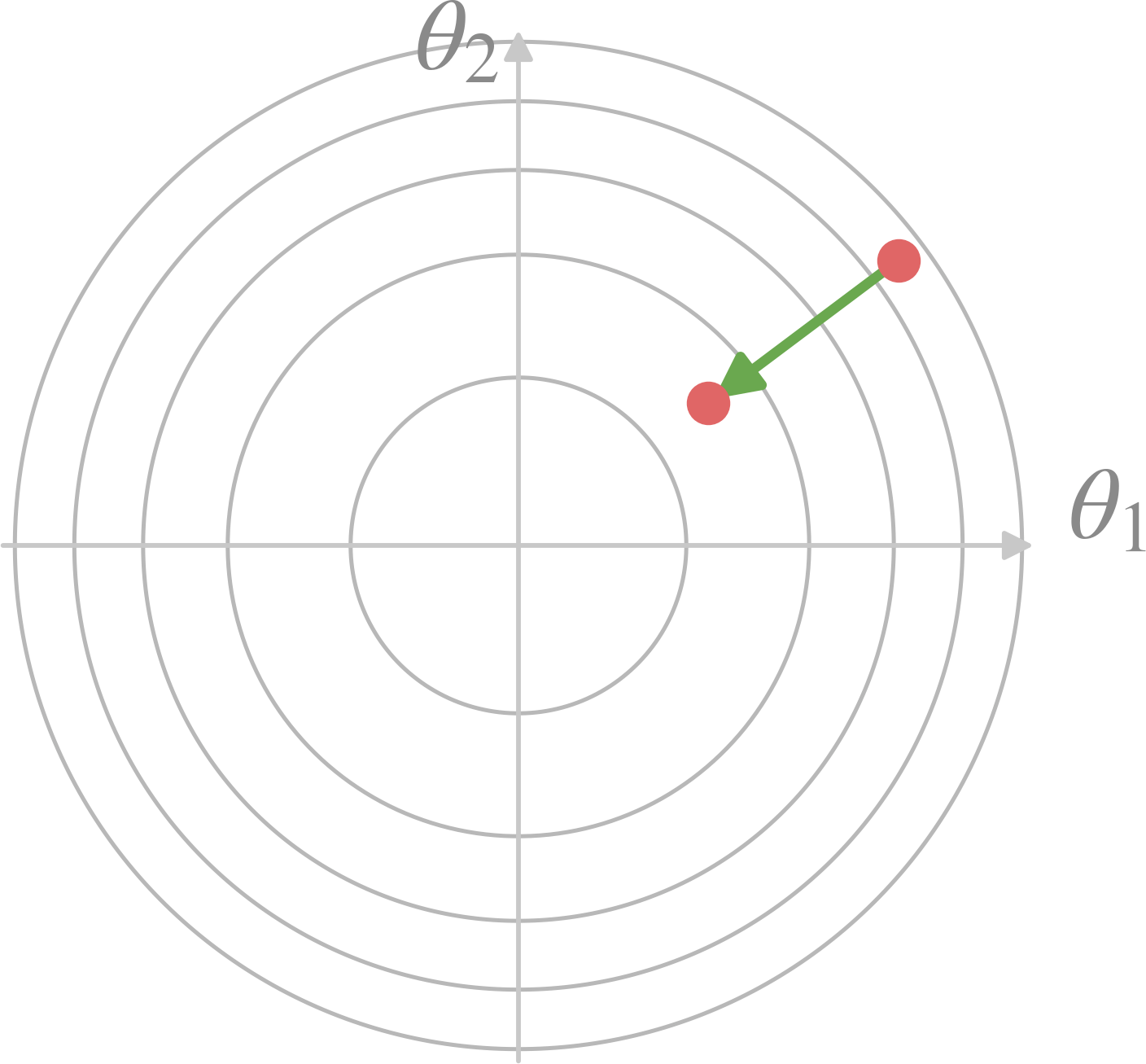
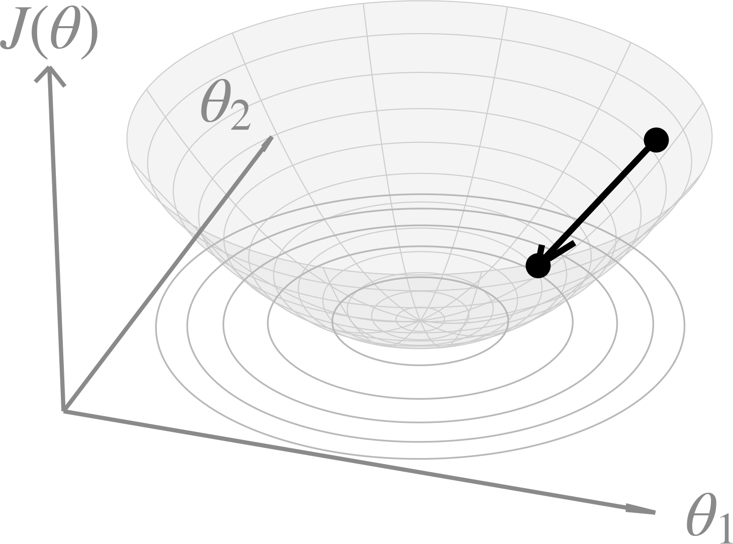
this 2d vector represents the step taken in line 5
this 3d vector isn't directly in the pseudocode;
- its 2d horizontal projection is the step taken in line 5
- its 1d vertical projection is the \(J\) change in line 6
Outline
-
Gradient descent (GD)
- The gradient vector
- GD algorithm
- Gradient descent properties
- Stochastic gradient descent (SGD)

When minimizing a function, we aim for a global minimizer.
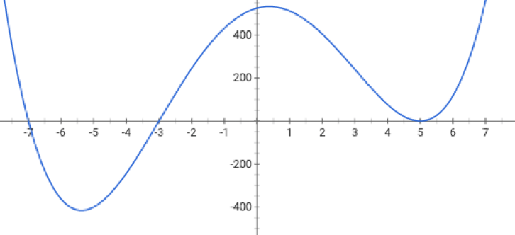



At a global minimizer
the gradient vector is zero
\(\Rightarrow\)
\(\nLeftarrow\)

gradient descent can achieve this (to arbitrary precision)
the gradient vector is zero
\(\Leftarrow\)
the objective function is convex
\{
A function \(f\) is convex if:
any line segment connecting two points of the graph of \(f\) lies above or on the graph.
- \(f\) is concave if \(-f\) is convex.
- Convex functions are the largest well-understood class of functions where optimization theory guarantees convergence and efficiency
When minimizing a function, we aim for a global minimizer.
At a global minimizer
- \(J_{\text{MSE}}\) is always convex
- \(J_{\text{ridge}}\) with \(\lambda >0\) is always (strongly) convex
convexity is why we can claim the point whose gradient is zero is a global minimizer.
More examples
Convex functions
Non-convex functions
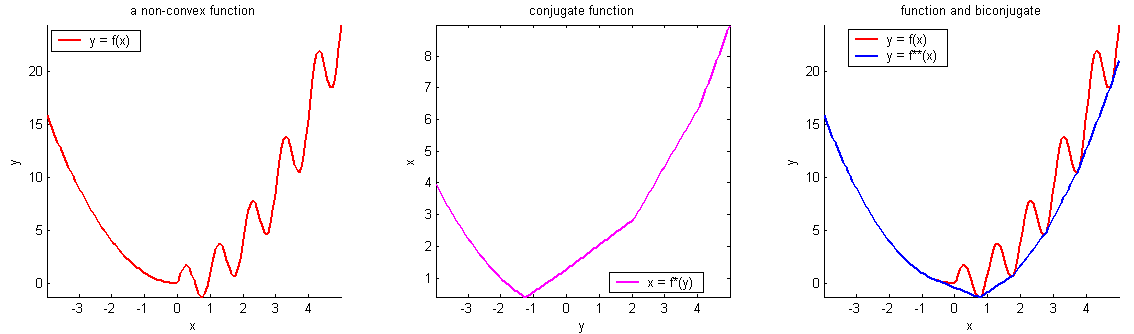
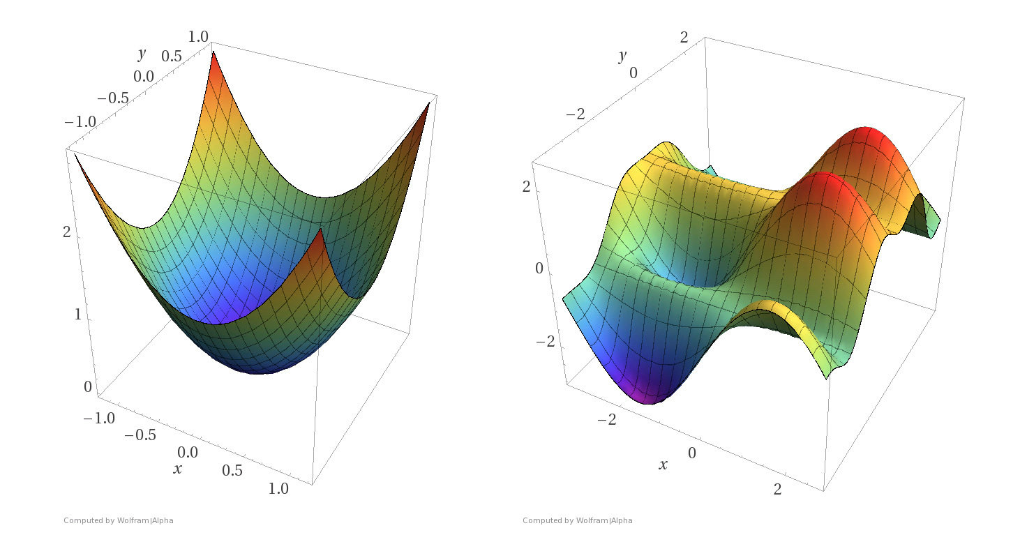
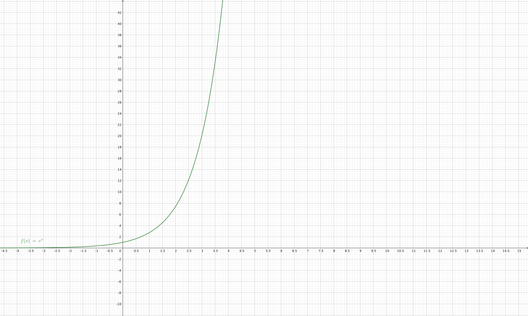
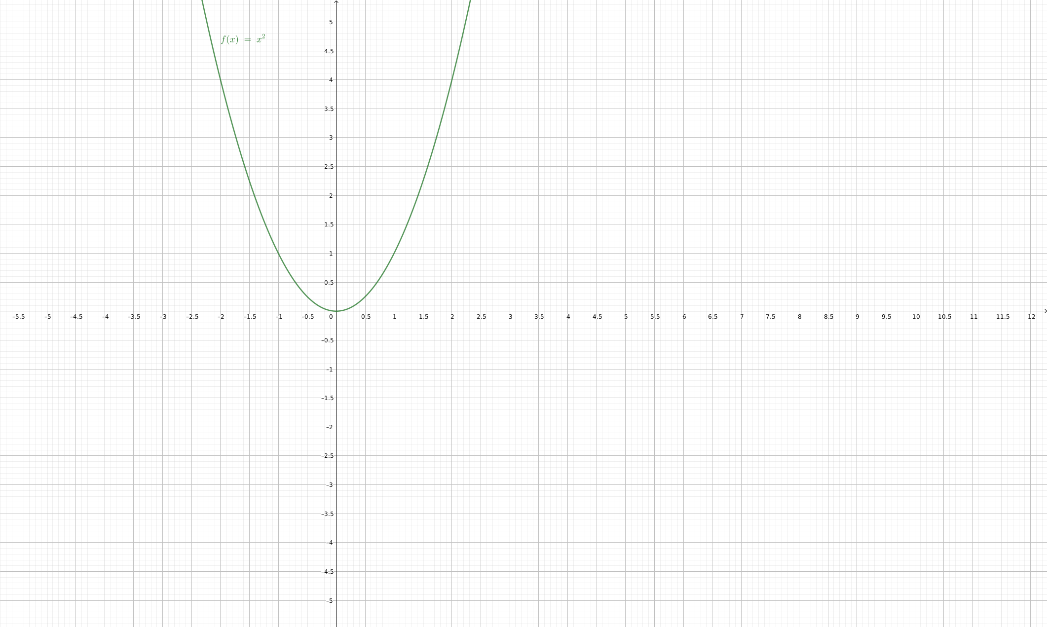

- Assumptions:
- \(f\) is sufficiently "smooth"
- \(f\) is convex
- \(f\) has at least one global minimum
- Run gradient descent for sufficient iterations
- \(\eta\) is sufficiently small
- Conclusion:
- Gradient descent converges arbitrarily close to a global minimizer of \(f\).
Gradient Descent Performance
if violated, may not have gradient,
can't run gradient descent
Gradient Descent Performance
- Assumptions:
- \(f\) is sufficiently "smooth"
- \(f\) is convex
- \(f\) has at least one global minimum
- Run gradient descent for sufficient iterations
- \(\eta\) is sufficiently small
- Conclusion:
- Gradient descent converges arbitrarily close to a global minimizer of \(f\).
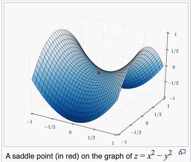
if violated, may get stuck at a saddle point
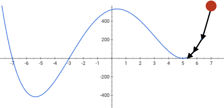
or a local minimum
- Assumptions:
- \(f\) is sufficiently "smooth"
- \(f\) is convex
- \(f\) has at least one global minimum
- Run gradient descent for sufficient iterations
- \(\eta\) is sufficiently small
- Conclusion:
- Gradient descent converges arbitrarily close to a global minimizer of \(f\).
Gradient Descent Performance
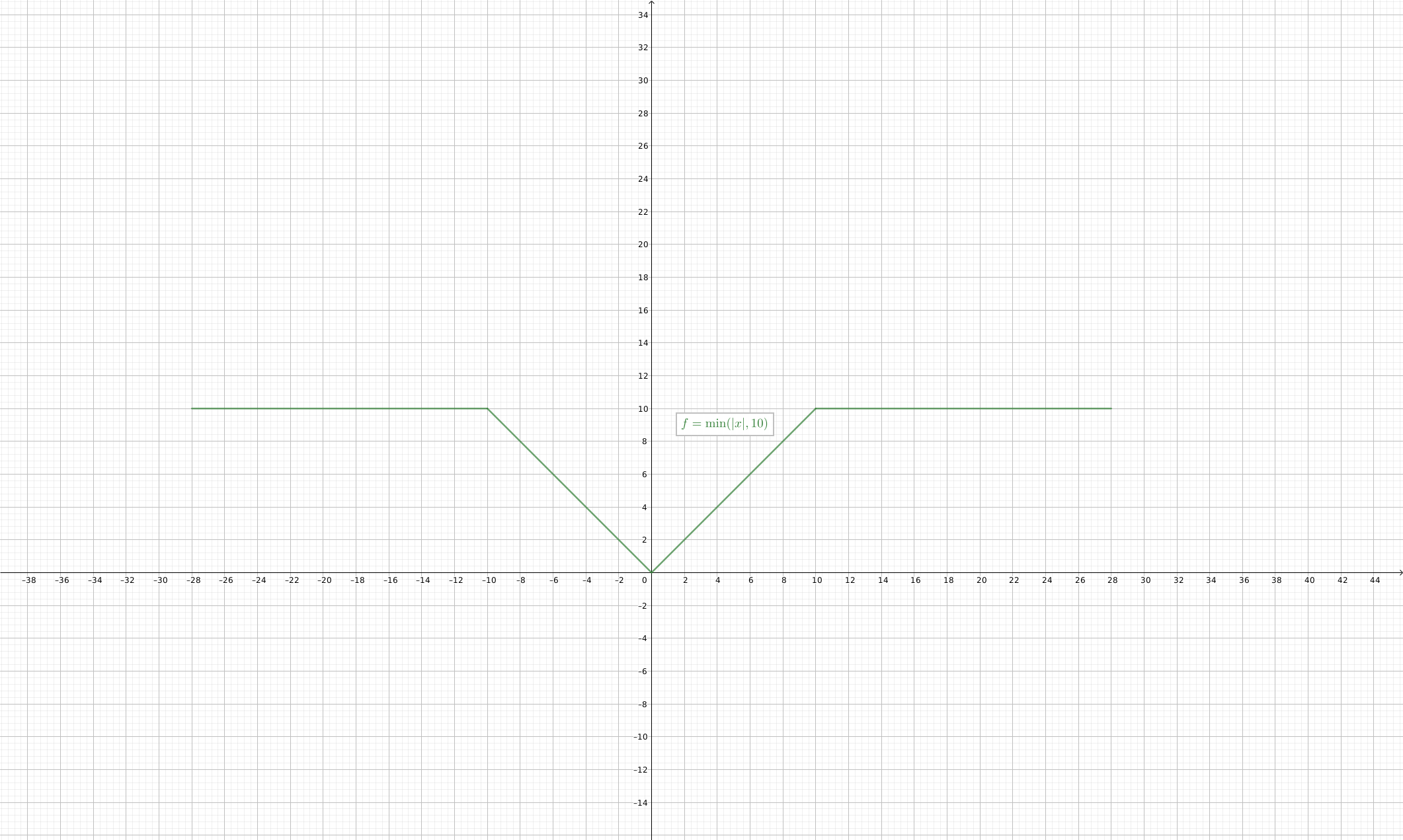
if violated:
may not terminate/no minimum to converge to
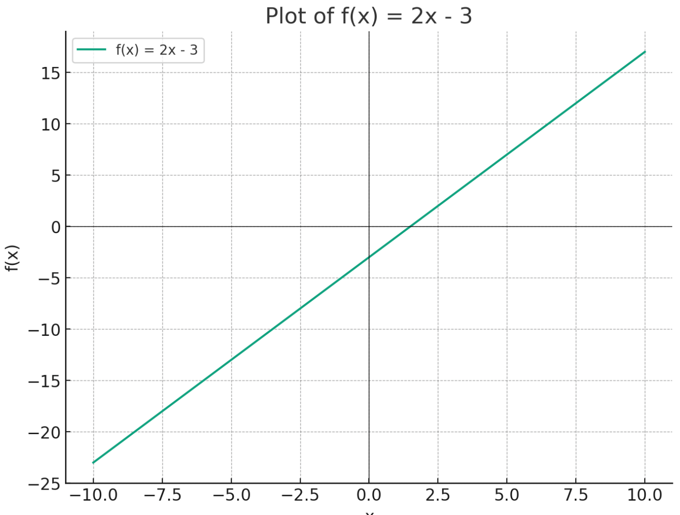
Gradient Descent Performance
- Assumptions:
- \(f\) is sufficiently "smooth"
- \(f\) is convex
- \(f\) has at least one global minimum
- Run gradient descent for sufficient iterations
- \(\eta\) is sufficiently small
- Conclusion:
- Gradient descent converges arbitrarily close to a global minimizer of \(f\).
Gradient Descent Performance
- Assumptions:
- \(f\) is sufficiently "smooth"
- \(f\) is convex
- \(f\) has at least one global minimum
- Run gradient descent for sufficient iterations
- \(\eta\) is sufficiently small
- Conclusion:
- Gradient descent converges arbitrarily close to a global minimizer of \(f\).
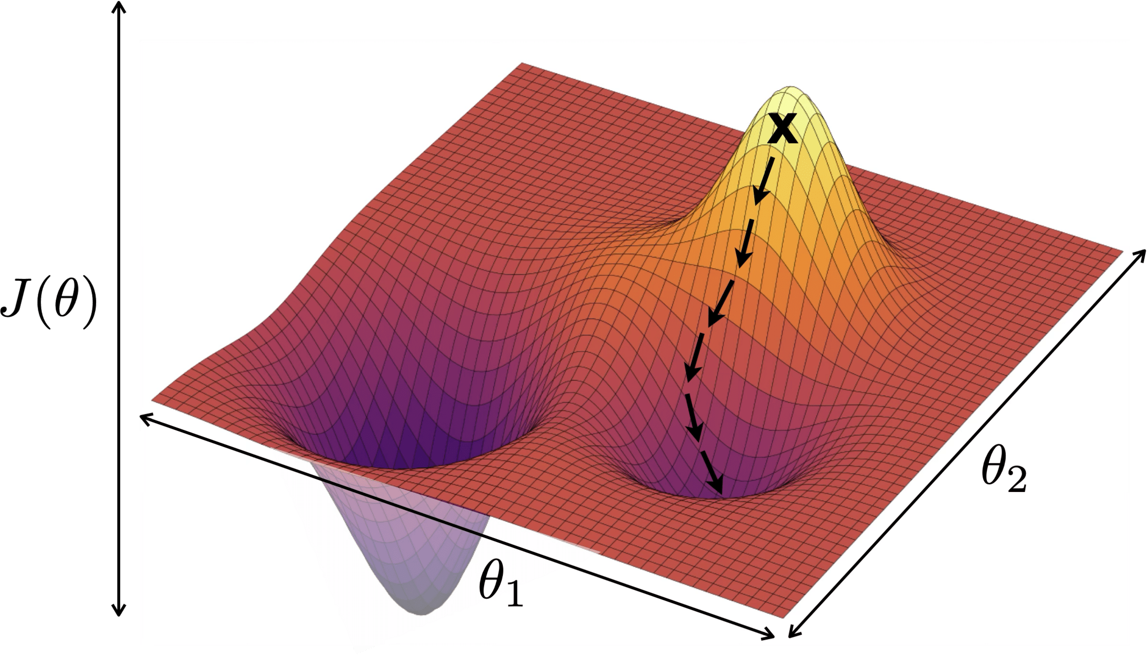
if violated:
see demo on next slide, also lab/hw
J(\theta)
\theta_1
\theta_2

Outline
- Gradient descent (GD)
-
Stochastic gradient descent (SGD)
- SGD algorithm and setup
- SGD vs. GD
Example 2: fit a line (no offset) to minimize MSE (3 data points)
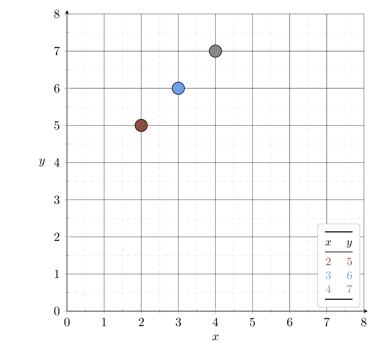
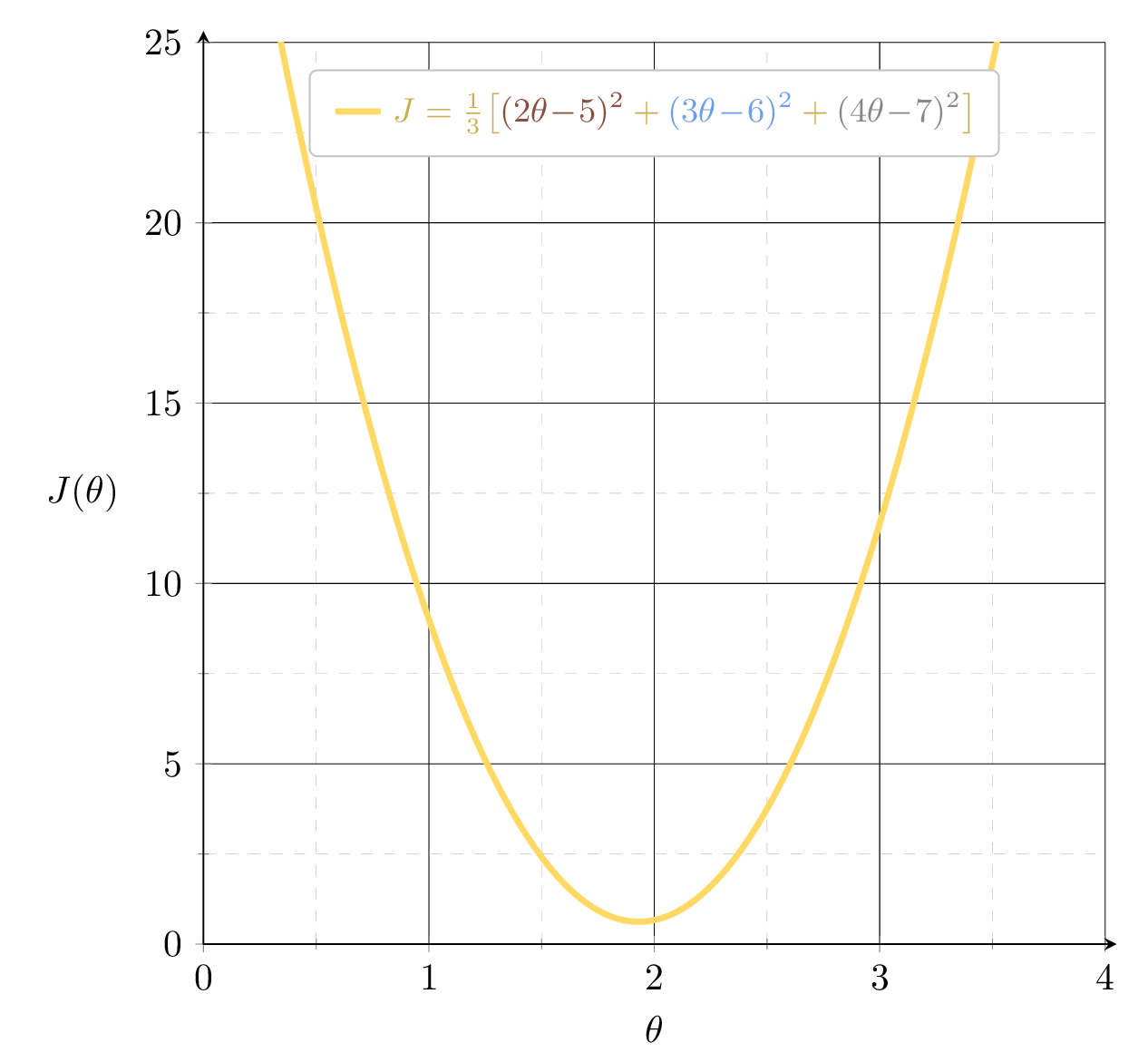
\(J_1 = (2\theta-5)^2\)
\(J_2 = (3\theta-6)^2\)
\(J_3 = (4\theta-7)^2\)
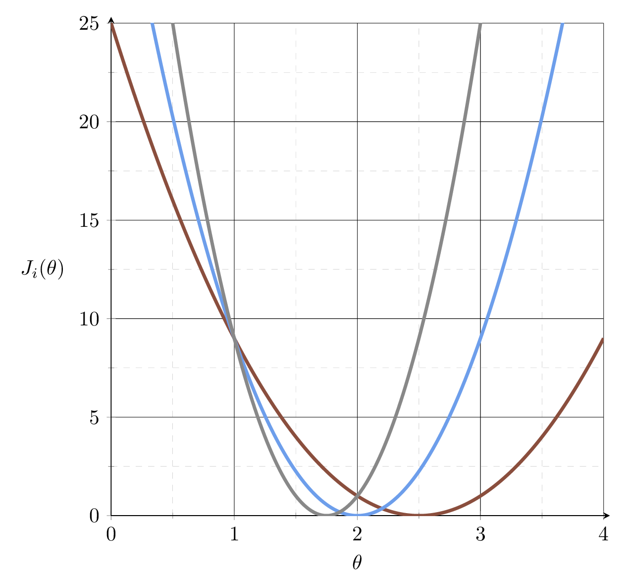
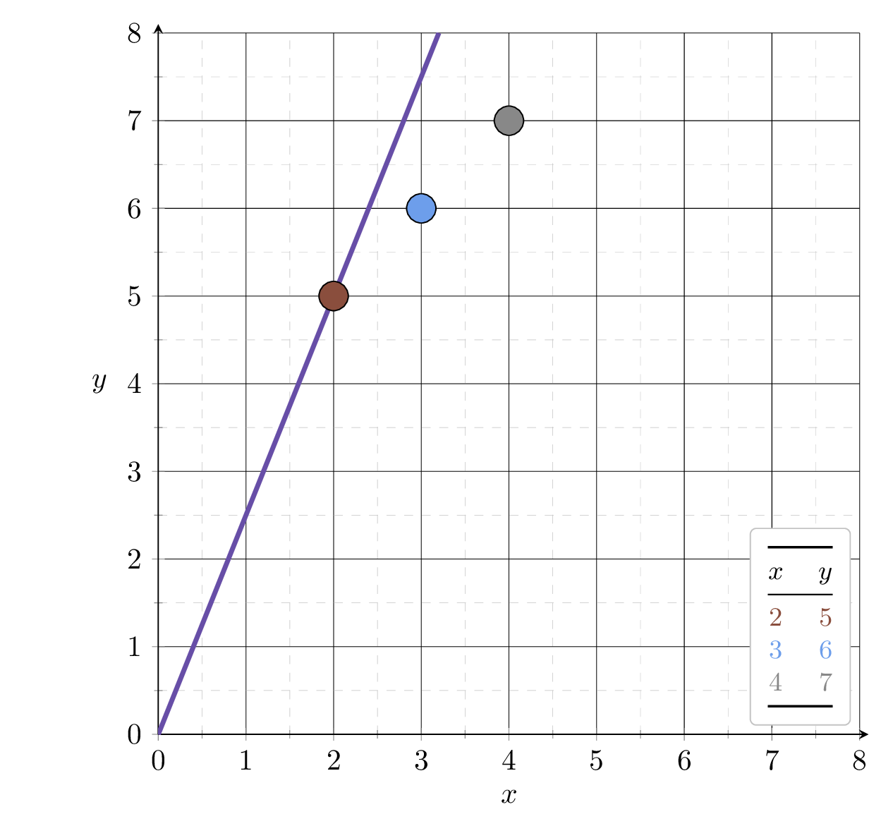
Suppose we fit \(h= 2.5x\)
MSE could get better, by leveraging the gradient
2.5
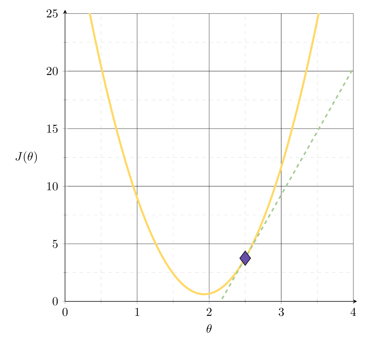
slope= 11
\(\nabla_\theta J = \frac{1}{3}\Big[\) \(\nabla_\theta J_1\) \(+\) \(\nabla_\theta J_2\) \(+\) \(\nabla_\theta J_3\) \(\Big]\)
slope \(= 0\)
slope \(= 9\)
slope \(= 24\)
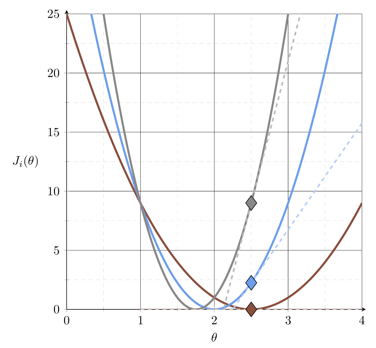
\(J_1 = (2\theta-5)^2\)
\(J_2 = (3\theta-6)^2\)
\(J_3 = (4\theta-7)^2\)
slope
\(= \frac{1}{3}(\)\(0\) \(+\) \(9\) \(+\) \(24\)\() \\ = 11\)
\(J = \frac{1}{3}\!\big[\)\((J_1\) \(+\) \(J_2\) \(+\) \(J_3\)\(\big]\)
Besides
we also have
slope= 11
At a different \(\theta =\begin{bmatrix} 1 \\ 1 \end{bmatrix}\)
Why is \(\nabla J_1 = 0?\)
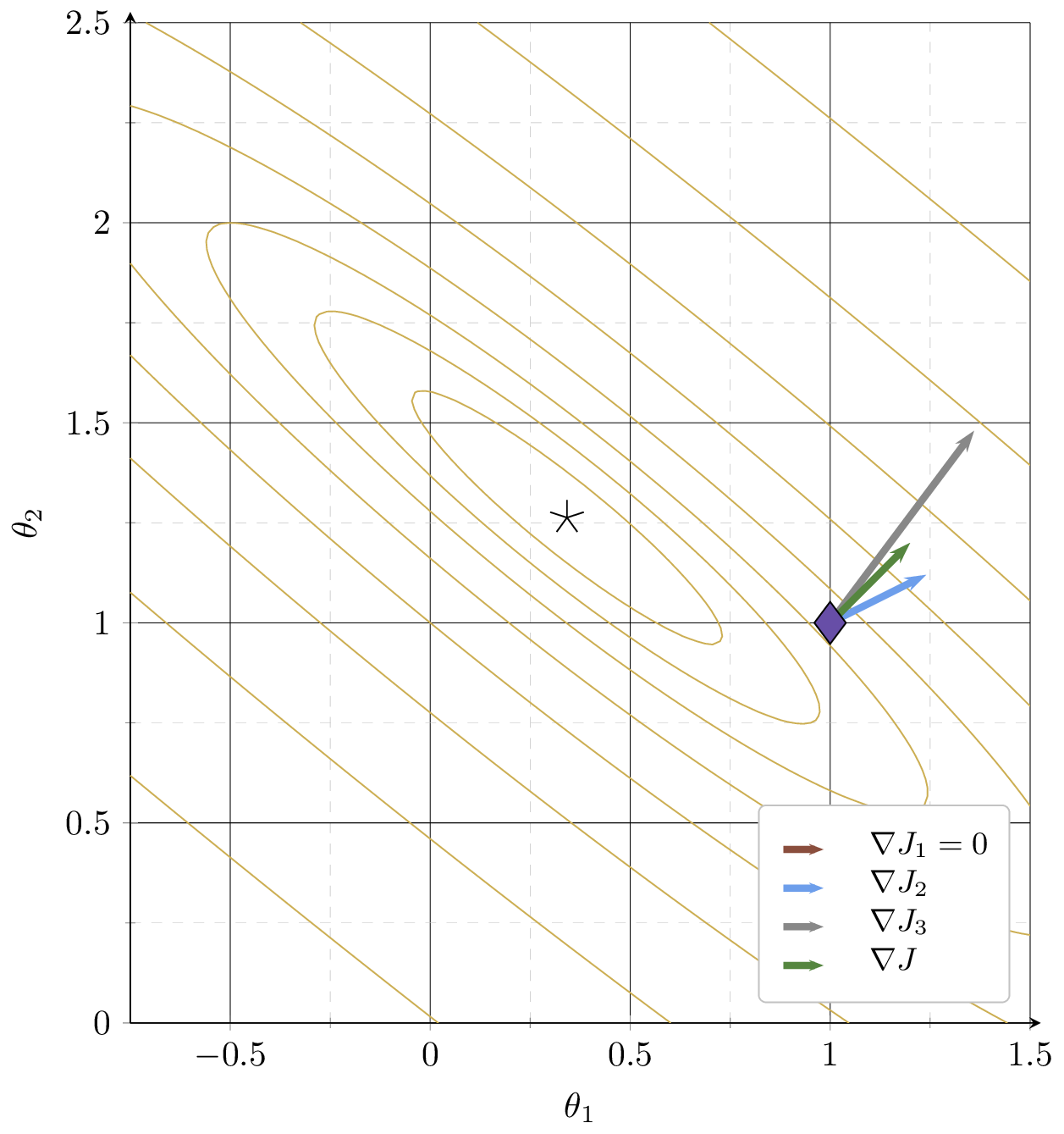
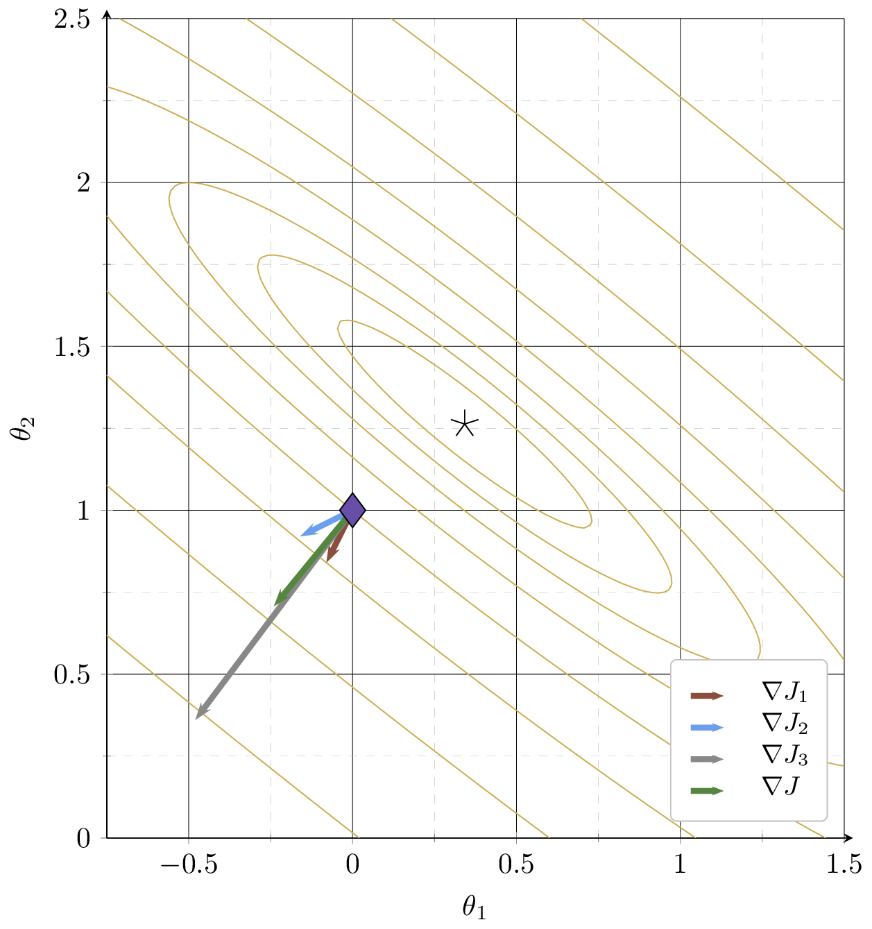
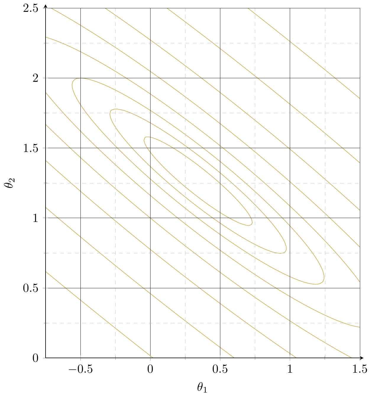
contours of \(J = \frac{1}{3}\!\big[\)\((3\!-\!\theta_1\!-\!2\theta_2)^2\) \(+\) \((2\!-\!2\theta_1\!-\!\theta_2)^2\) \(+\) \((6\!-\!3\theta_1\!-\!4\theta_2)^2\)\(\big]\)
\( = \frac{1}{3}\!\big[\)\((J_1\) \(+\) \(J_2\) \(+\) \(J_3\)\(\big]\)
Example 3:
training data set
| \(x_1\) | \(x_2\) | \(y\) |
| 1 | 2 | 3 |
| 2 | 1 | 2 |
| 3 | 4 | 6 |
Gradient of an ML objective
- An ML objective function is a finite sum
- and its gradient w.r.t. \(\theta\):
\nabla_\theta J(\theta) = \nabla (\frac{1}{n} \sum_{i=1}^n J_i(\theta))
\nabla_\theta J(\theta) = \frac{1}{n} \sum_{i=1}^n2\left(\theta^{\top} x^{(i)}-y^{(i)}\right) x^{(i)}
= \frac{1}{n} \sum_{i=1}^n \nabla_\theta J_i(\theta)
In general,
J(\theta) = \frac{1}{n} \sum_{i=1}^n\left(\theta^{\top} x^{(i)}-y^{(i)}\right)^2
J(\theta)=\frac{1}{n} \sum_{i=1}^n J_i(\theta)
👋 (gradient of the sum) = (sum of the gradient)
👆
- the MSE of a linear hypothesis:
- and its gradient w.r.t. \(\theta\):
Gradient of an ML objective
- An ML objective function is a finite sum
- and its gradient w.r.t. \(\theta\):
\nabla_\theta J(\theta) = \nabla (\frac{1}{n} \sum_{i=1}^n J_i(\theta))
= \frac{1}{n} \sum_{i=1}^n \nabla_\theta J_i(\theta)
In general,
J(\theta)=\frac{1}{n} \sum_{i=1}^n J_i(\theta)
gradient info from the \(i^{\text{th}}\) data point's loss
need to add \(n\) of these, each\(\nabla_\theta J_i\in \mathbb{R}^{d}\)
loss incurred on a single \(i^{\text{th}}\) data point
Costly in practice!
\nabla_\theta J(\theta)
\approx \nabla_\theta J_i(\theta)
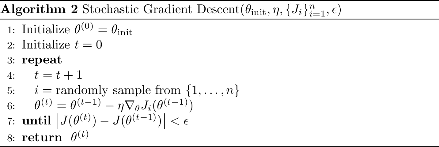
= \frac{1}{n} \sum_{i=1}^n \nabla_\theta J_i(\theta)
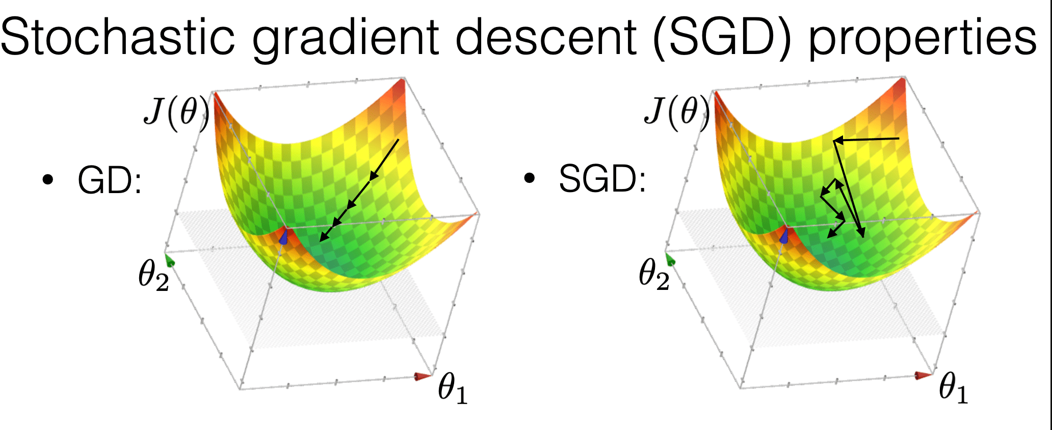
is much noisier
is cheaper per step
may get us out of a local minimum
Compared with GD, SGD
\nabla_\theta J(\theta)
\approx \nabla_\theta J_i(\theta)
= \frac{1}{n} \sum_{i=1}^n \nabla_\theta J_i(\theta)
Stochastic gradient descent performance
- Assumptions:
- \(f\) is sufficiently "smooth"
- \(f\) is convex
- \(f\) has at least one global minimum
- Run gradient descent for sufficient iterations
- \(\eta\) is sufficiently small and satisfies additional "scheduling" condition1
- Conclusion:
- Stochastic gradient descent converges arbitrarily close to a global minimum of \(f\) with probability 1.
¹ \(\sum_{t=1}^{\infty} \eta(t)=\infty\) and \(\sum_{t=1}^{\infty} \eta(t)^2<\infty\), e.g., \(\eta(t) = 1/t\)
See Robbins & Monro “A Stochastic Approximation Method” for more details
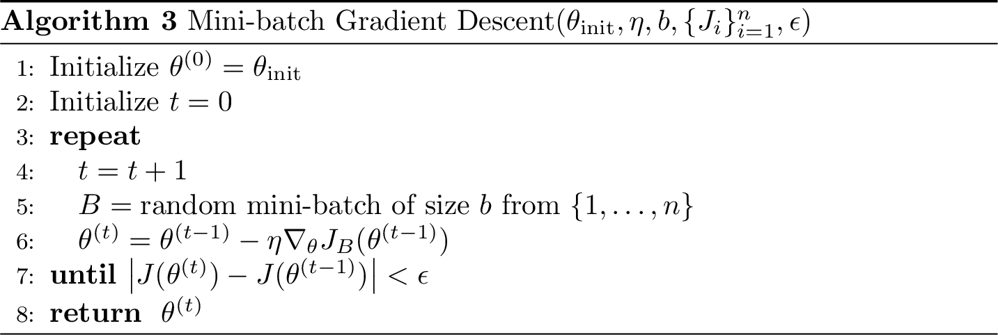
\frac{1}{b} \sum_{i=1}^b \nabla_\theta J_i(\theta)
batch size
🥰more accurate gradient, stronger theoretical guarantee
🥺more costly per parameter update step
mini-batch GD
\frac{1}{n} \sum_{i=1}^n \nabla_\theta J_i(\theta)= \nabla_\theta J(\theta)
GD
\nabla_\theta J_i(\theta)
SGD
Summary
-
Most ML problems require optimization; closed-form solutions don't always exist or scale.
-
Gradient descent iteratively updates \(\theta\) in the direction of steepest descent of \(J\).
-
With a convex \(J\) and small enough \(\eta\), GD converges to a global minimum.
-
SGD follows one data point's gradient, so each step is noisy but cheap.
-
Mini-batch averages a small batch of data points' gradients; it achieves the practical middle ground and is the default in modern practice.
\(\theta^{(t)} = \theta^{(t-1)} - \eta\, \nabla_\theta J(\theta^{(t-1)})\)
6.390 IntroML (Fall26) - Lecture 3 Gradient Descent Methods
By Shen Shen