
Lecture 7: Convolutional Neural Networks
Intro to Machine Learning

\dots
layer
linear combo
activations
\dots
\dots
layer
\dots
x_1
x_2
x_d
input
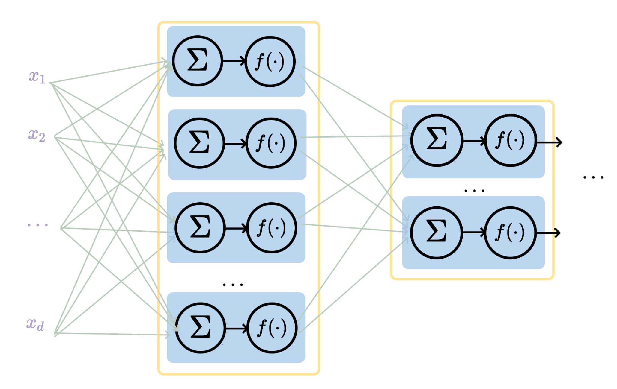
\Sigma
f(\cdot)
\Sigma
f(\cdot)
\Sigma
f(\cdot)
\Sigma
f(\cdot)
\Sigma
f(\cdot)
\Sigma
f(\cdot)
\Sigma
f(\cdot)
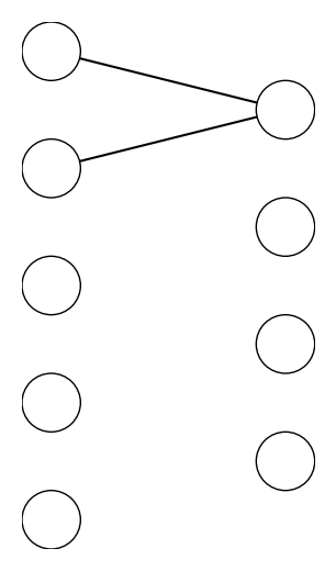
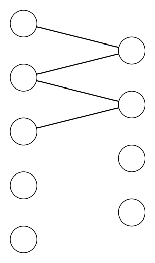
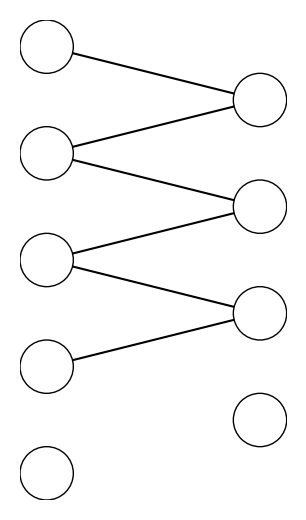
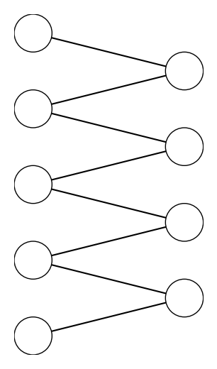
neuron
learnable weights
hidden
output
a (fully-connected, feed-forward) neural network
Recap
x^{(1)}
y^{(1)}
f^1
\begin{aligned}
& W^1 \\
\end{aligned}
\begin{aligned}
& W^2 \\
\end{aligned}
\begin{aligned}
& W^L \\
\end{aligned}
f^2
f^L
g^{(1)}
\(\dots\)
f^2\left(\hspace{2cm}; \mathbf{W}^2\right)
f^1(\mathbf{x}^{(i)}; \mathbf{W}^1)
f^L\left(\dots \hspace{3.5cm}; \dots \mathbf{W}^L\right)
Forward pass: evaluate, given the current parameters
- the model outputs \(g^{(i)}\) =
- the loss incurred on the current data \(\mathcal{L}(g^{(i)}, y^{(i)})\)
- the training error \(J = \frac{1}{n} \sum_{i=1}^{n}\mathcal{L}(g^{(i)}, y^{(i)})\)
\mathcal{L}(g^{(1)}, y^{(1)})
\mathcal{L}(g, y)
\mathcal{L}(g^{(n)}, y^{(n)})
\underbrace{\quad \quad \quad \quad \quad }
\dots
\dots
\dots
n
linear combination
loss function
(nonlinear) activation
Recap
- Randomly pick a data point \((x^{(i)}, y^{(i)})\)
- Evaluate the gradient \(\nabla_{W^2} \mathcal{L}(g^{(i)},y^{(i)})\)
- Update the weights \(W^2 \leftarrow W^2 - \eta \nabla_{W^2} \mathcal{L}(g^{(i)},y^{(i)})\)
x^{(i)}
y^{(i)}
f^1
\begin{aligned}
& W^1 \\
\end{aligned}
\begin{aligned}
& W^2 \\
\end{aligned}
\begin{aligned}
& W^L \\
\end{aligned}
f^2
f^L
g^{(i)}
\(\dots\)
\mathcal{L}(g^{(i)}, y^{(i)})
\mathcal{L}(g, y)
\mathcal{L}(g^{(n)}, y^{(n)})
\underbrace{\quad \quad \quad \quad \quad }
\dots
\dots
\dots

\(\nabla_{W^2} \mathcal{L}(g^{(i)},y^{(i)})\)
n
Backward pass: run SGD to update all parameters
e.g. to update \(W^2\)
Recap
\underbrace{\hspace{6.5cm}}
\frac{\partial Z^2}{\partial A^{1}}
\frac{\partial A^1}{\partial Z^{1}}
\frac{\partial Z^1}{\partial W^{1}}
x
\(\dots\)
y
f^1
\begin{aligned}
& W^1 \\
\end{aligned}
\begin{aligned}
& W^2 \\
\end{aligned}
\begin{aligned}
& W^L \\
\end{aligned}
f^2
f^L
\mathcal{L}(g,y)
g
Z^L
A^2
Z^2
A^1
Z^1
\frac{\partial \mathcal{L}}{\partial W^1} = \frac{\partial Z^1}{\partial W^1} \cdot \frac{\partial A^1}{\partial Z^1} \cdot \frac{\partial Z^2}{\partial A^1} \cdot \color{#93c47d}{\frac{\partial \mathcal{L}}{\partial Z^2}}
\underbrace{\hspace{4.7cm}}
\frac{\partial Z^2}{\partial W^{2}}
\frac{\partial \mathcal{L}}{\partial W^2} = \frac{\partial Z^2}{\partial W^2} \cdot \color{#93c47d}{\frac{\partial \mathcal{L}}{\partial Z^2}}
backpropagation: reuse of computation
\frac{\partial \mathcal{L}(g,y)}{\partial g}
\frac{\partial g}{\partial Z^{L}}
\frac{\partial Z^3}{\partial A^{2}}\frac{\partial A^3}{\partial Z^{3}} \dots \frac{\partial Z^L}{\partial A^{L-1}}
\frac{\partial \mathcal{L}(g,y)}{\partial Z^2}
\underbrace{\hspace{4cm}}
\frac{\partial A^2}{\partial Z^{2}}
Recap
convolutional neural networks
-
Why do we need a special network for images?
-
Why is CNN (the) special network for images?
9
Outline
- Vision problem structure
- Convolution
- 1-dimensional and 2-dimensional convolution
- 3-dimensional tensors
- Max pooling
- (Case studies)
[video edited from 3b1b]
Why do we need a specialized network (hypothesis class)?

For higher-resolution images, or more complex tasks, or larger networks, the number of parameters can grow very fast.
- Partly, fully-connected nets don't scale well for vision tasks
- More importantly, a carefully chosen hypothesis class helps fight overfitting
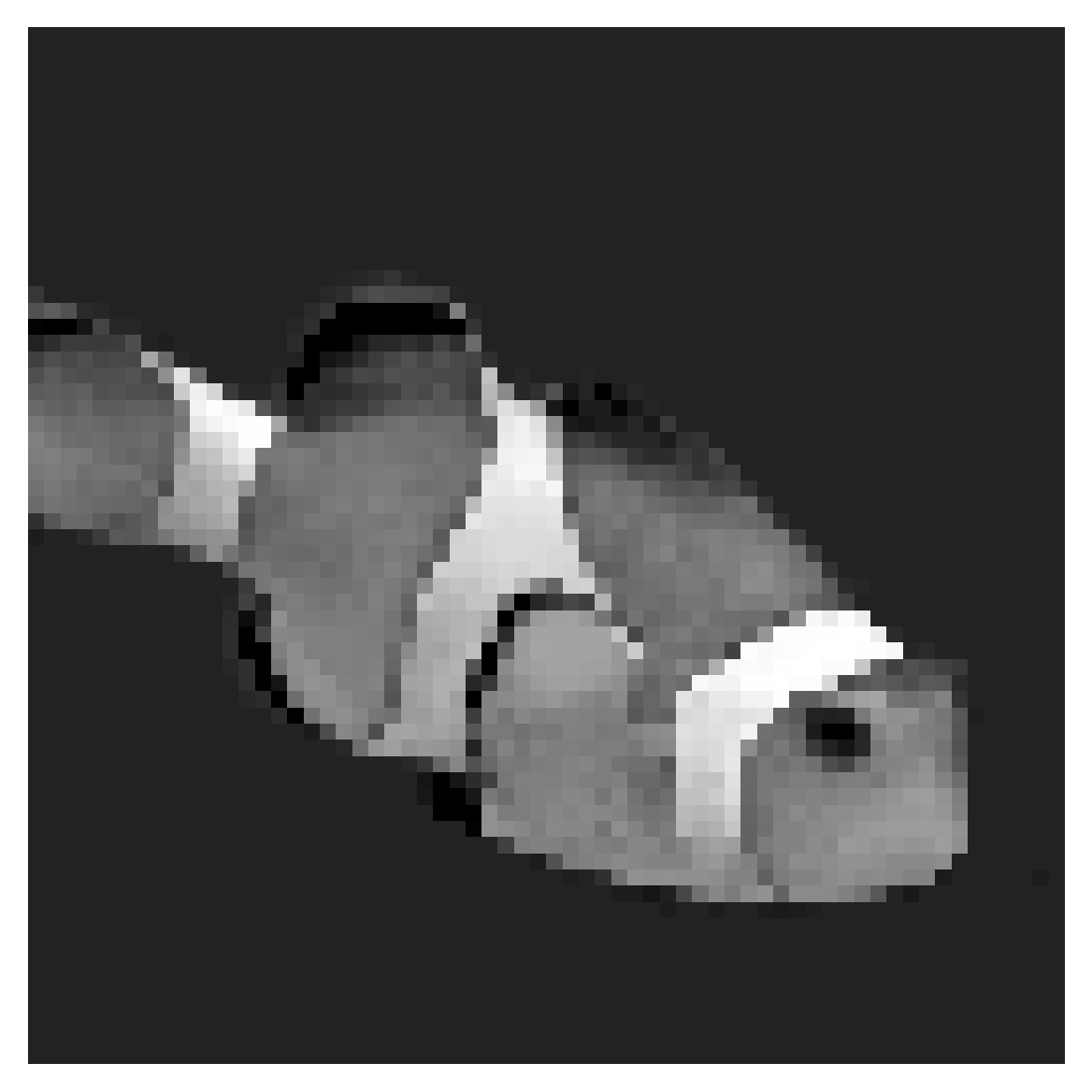
426-by-426 grayscale image
Use the same 2 hidden-layer network to predict what top-10 engineering school seal this image is, need to learn ~3M parameters.
Underfitting
Appropriate
Overfitting
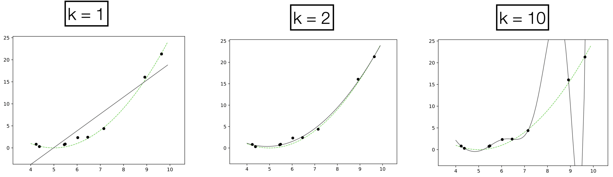
k=1
k=2
k=10
Recall, models with needless parameters tend to overfit
If we know the data is generated by the green curve, it's easy to choose the appropriate quadratic hypothesis class.
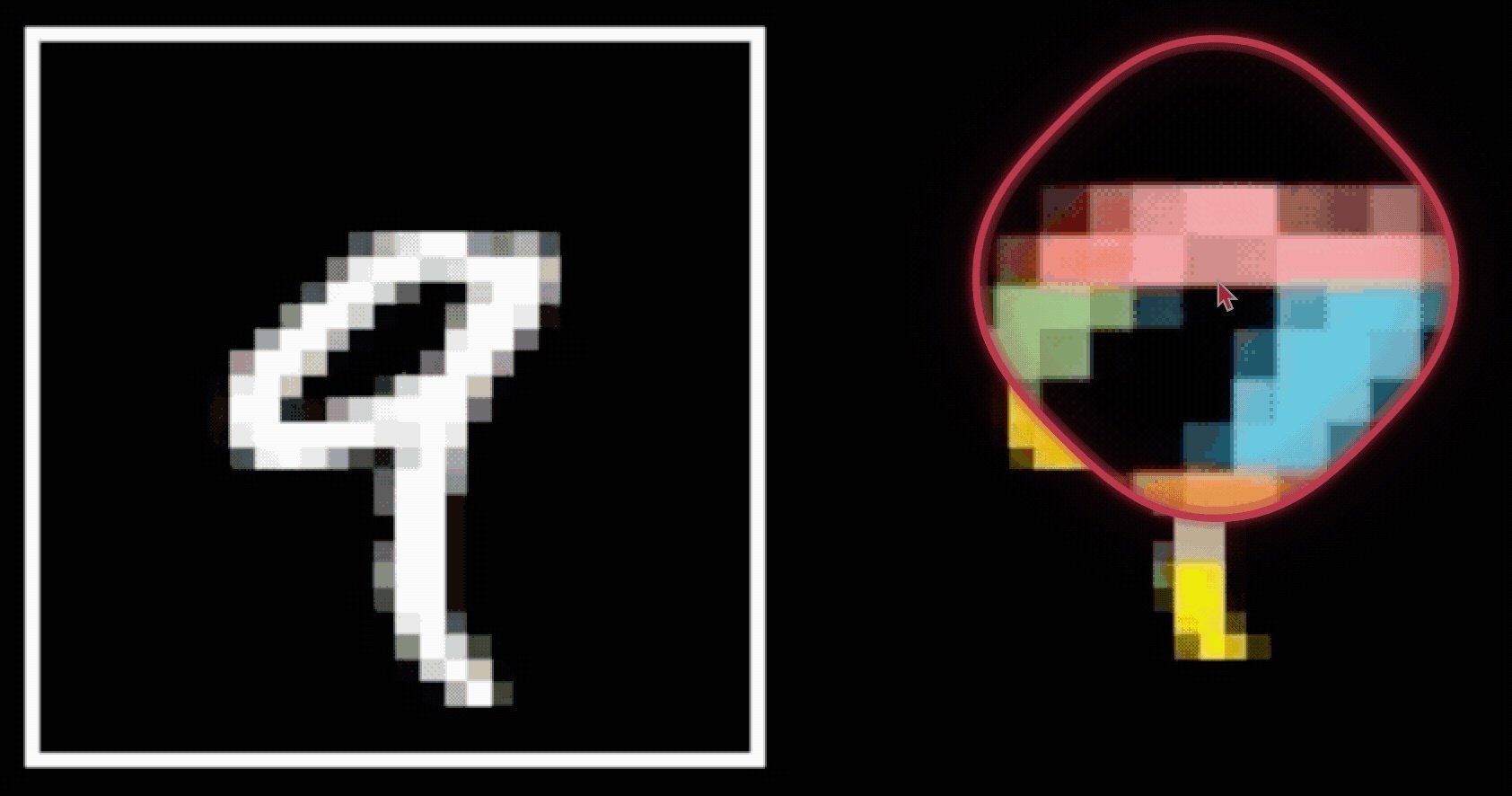
so... do we know anything about vision problems?
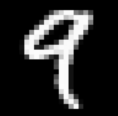
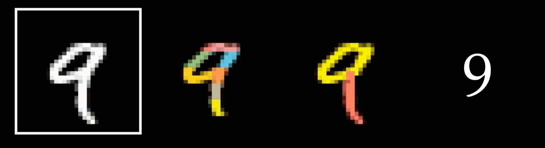
Why do we humans think
is a 9?

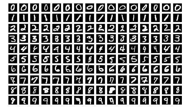
Why do we think any of
is a 9?
[video edited from 3b1b]
- Visual hierarchy
Layered structure are well-suited to model this hierarchical processing.
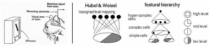
- Visual hierarchy
- Spatial locality
- Translational invariance
CNN exploits
to handle images efficiently and effectively.
via
- layered structure
- convolution
- pooling
- Visual hierarchy
- Spatial locality
- Translational invariance
CNN
the same feedforward net as before
\underbrace{\hspace{6cm}}
typical CNN architecture for image classification
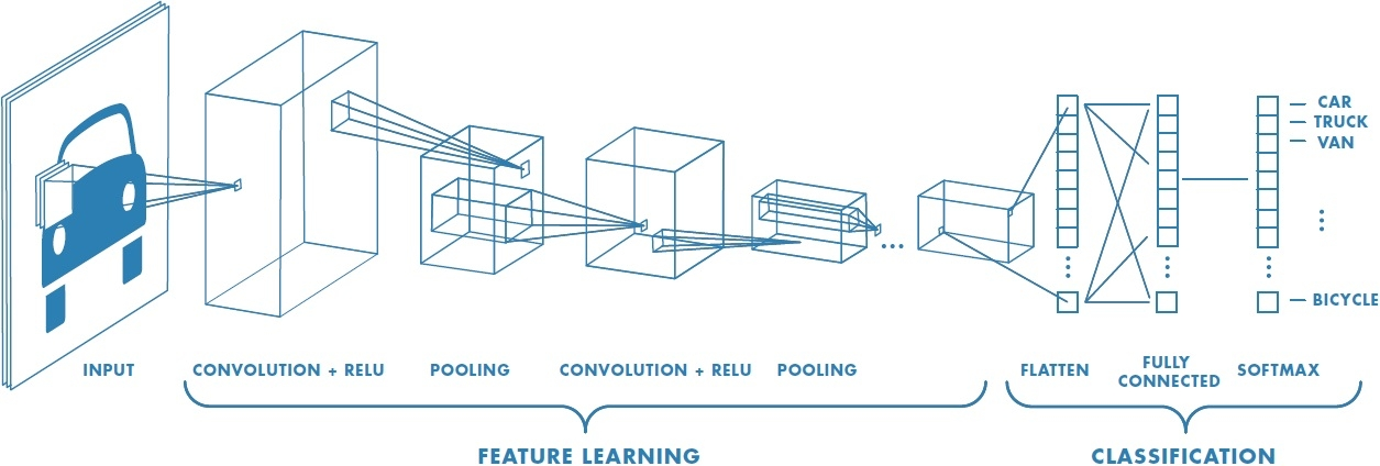
CNN
typical CNN structure for image classification
Outline
- Vision problem structure
-
Convolution
- 1-dimensional and 2-dimensional convolution
- 3-dimensional tensors
- Max pooling
- (Case studies)
Convolutional layer might sound foreign, but it's very similar to a fully-connected layer
Convolution result:
filter weights
convolution, activation
dot-product, activation
Forward pass, do
Backward pass, learn
neuron weights
Design choices
neuron count, etc.
| Layer | |||
|---|---|---|---|
| fully-connected | |||
| convolutional |
conv specs, etc.
0
1
0
1
1
-1
1
input
filter
convolved output
1
(0*-1)+(1*1)=1
example: 1-dimensional convolution
0
1
0
1
1
-1
1
input
filter
convolved output
1
(1*-1)+(0*1)=-1
-1
example: 1-dimensional convolution
0
1
0
1
1
-1
1
input
filter
convolved output
1
1
example: 1-dimensional convolution
(0*-1)+(1*1)=1
-1
0
1
0
1
1
-1
1
input
filter
convolved output
1
1
-1
(1*-1)+(1*1)=0
0
example: 1-dimensional convolution
0
1
-1
1
1
-1
1
input
filter
convolved output
template matching
1
-2
2
0
convolution interpretation 1:
-1
1
-1
1
-1
1
-1
1
convolution interpretation 2:
0
1
-1
1
1
-1
1
input
filter
convolved output
1
-2
2
0
"look" locally through the filter
this local region = receptive field
0
1
-1
1
1
1
-2
2
0
input
output
0
1
-1
1
1
-1
1
convolve with
=
dot product with
1
-2
2
0
1
0
0
0
0
-1
0
0
0
0
0
1
0
0
0
1
-1
0
1
-1
-1
convolution interpretation 3:
sparse-connected layer with parameter sharing
0
1
0
1
1
convolve with
dot product with
0
1
0
1
1
?
?
1
I_{5\times5}
| 0 | 1 |
convolution interpretation 4:
input
filter
convolved output
| 0 | 1 | 0 | 1 | 0 |
| 1 | 0 | 1 | 0 |
translational equivariance
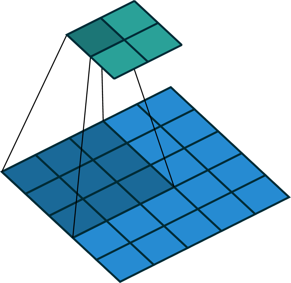
input
filter
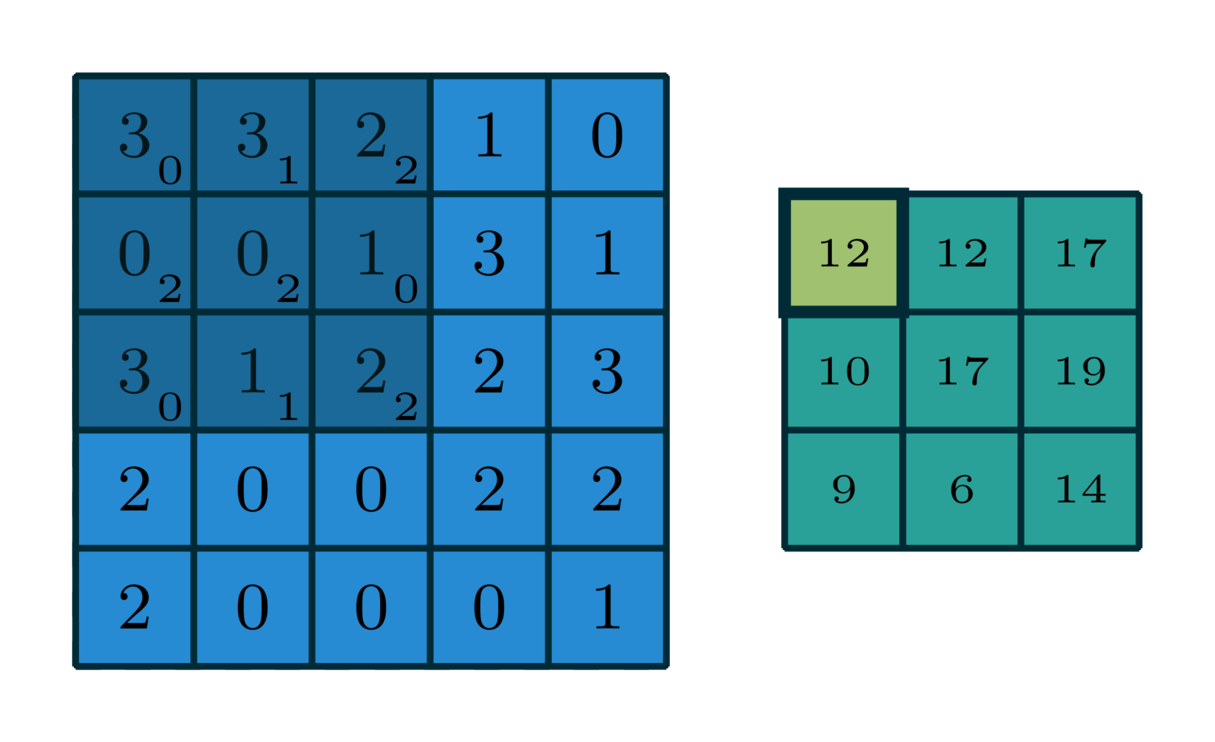
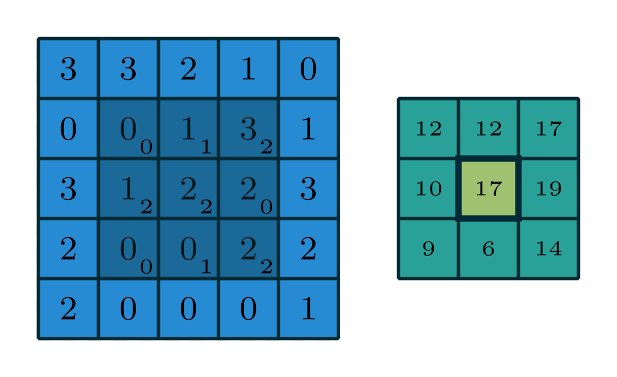
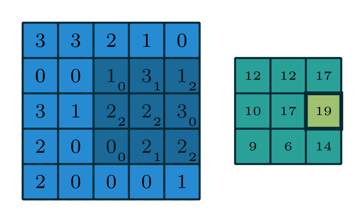
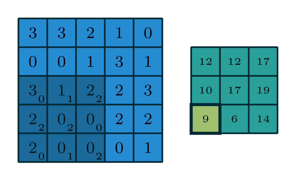
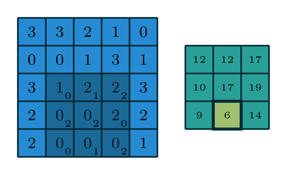
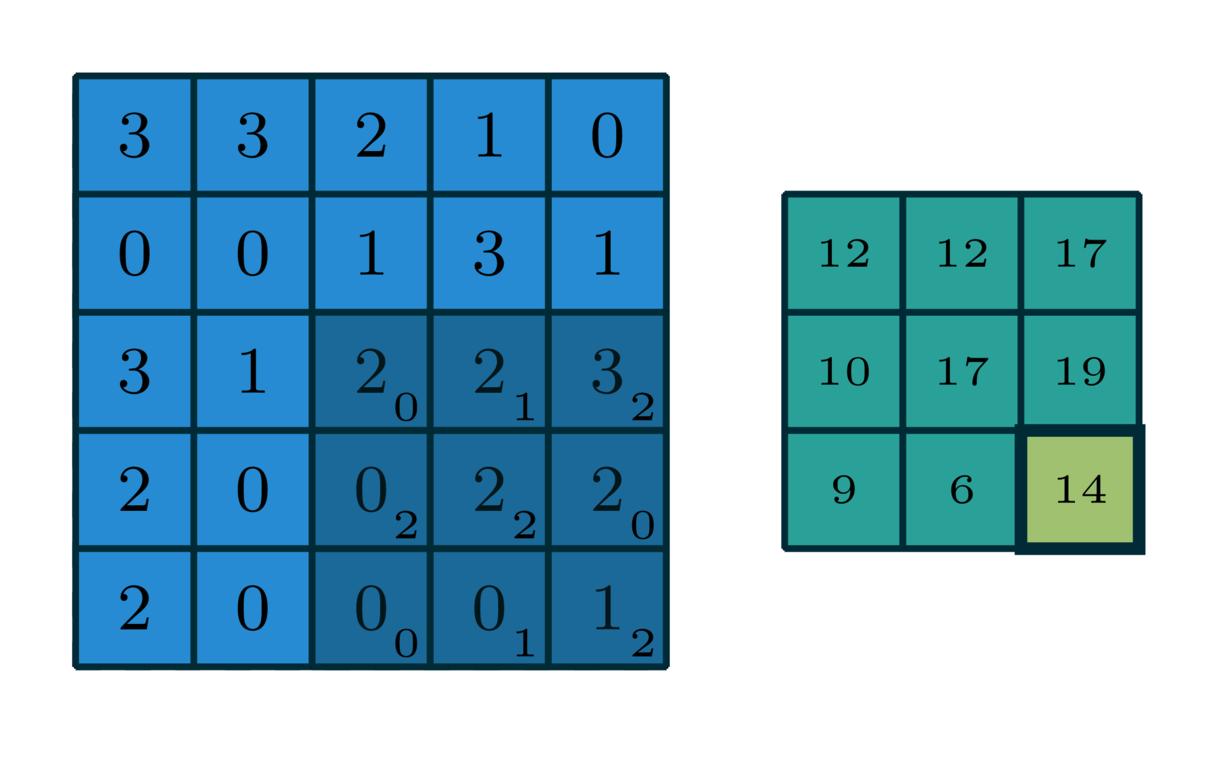
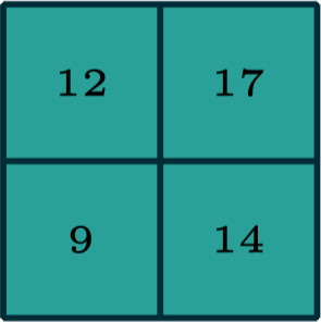
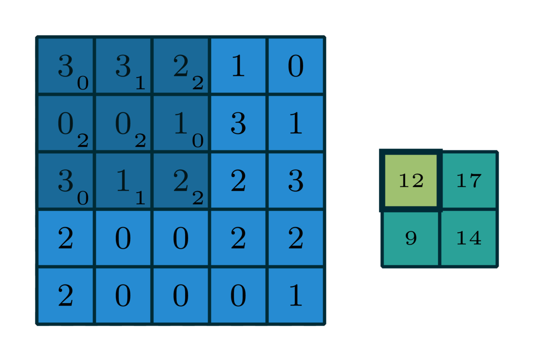
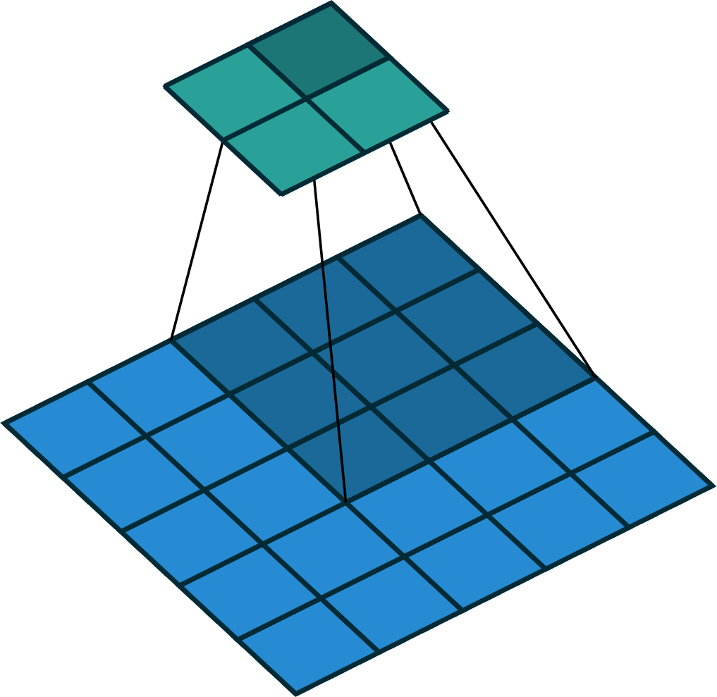
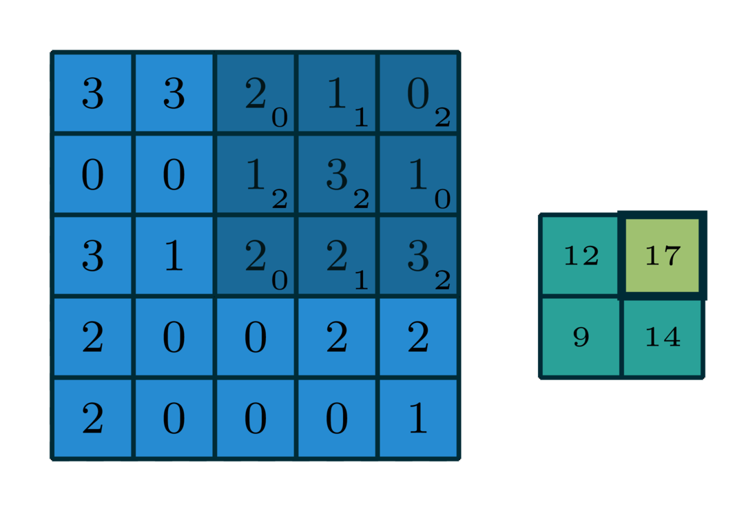
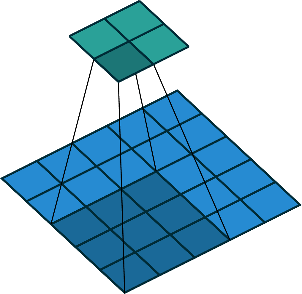
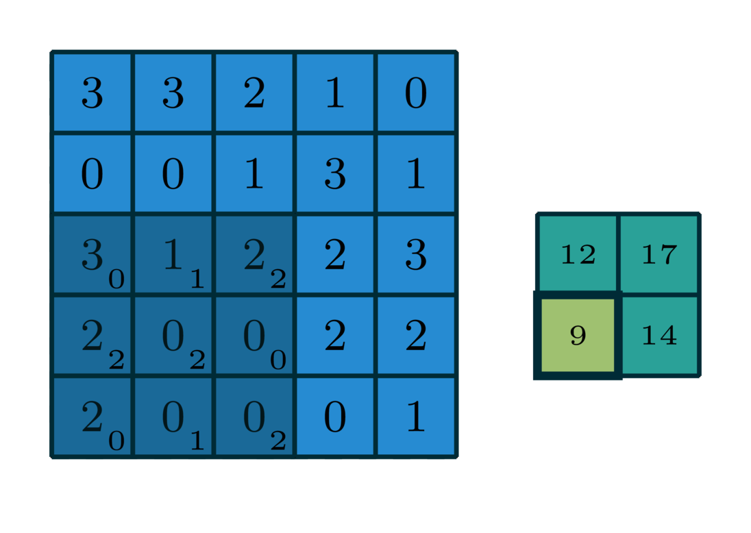
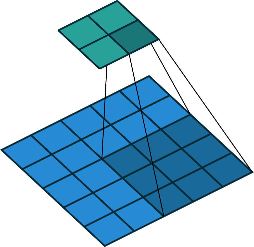
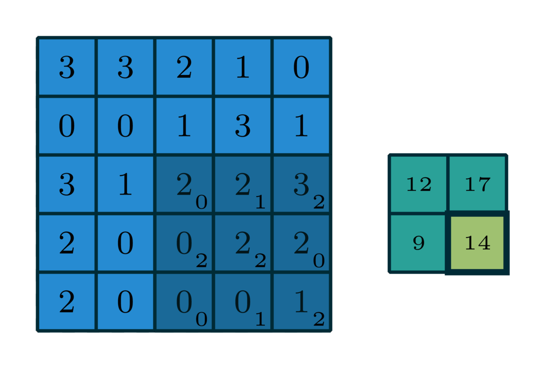
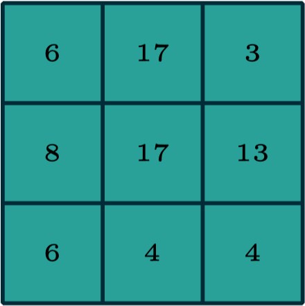
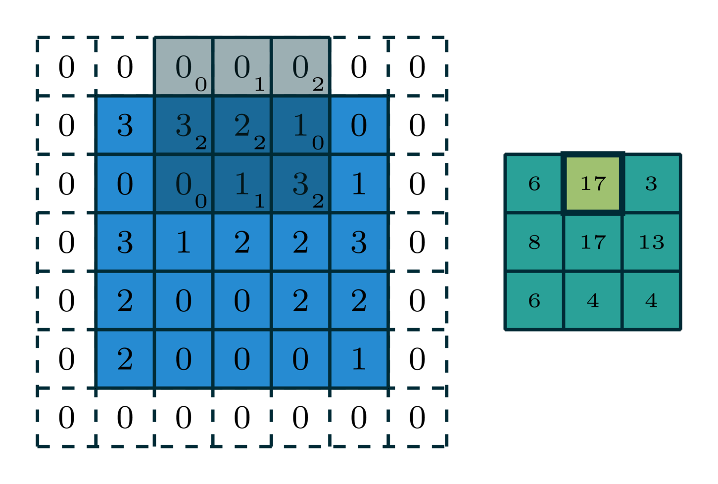
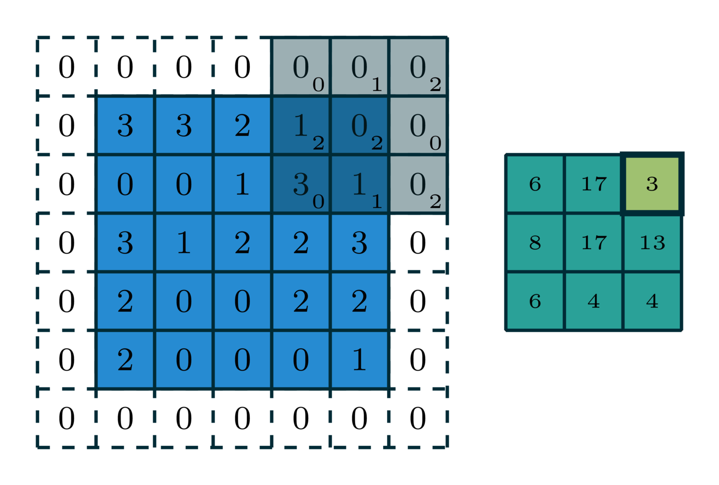
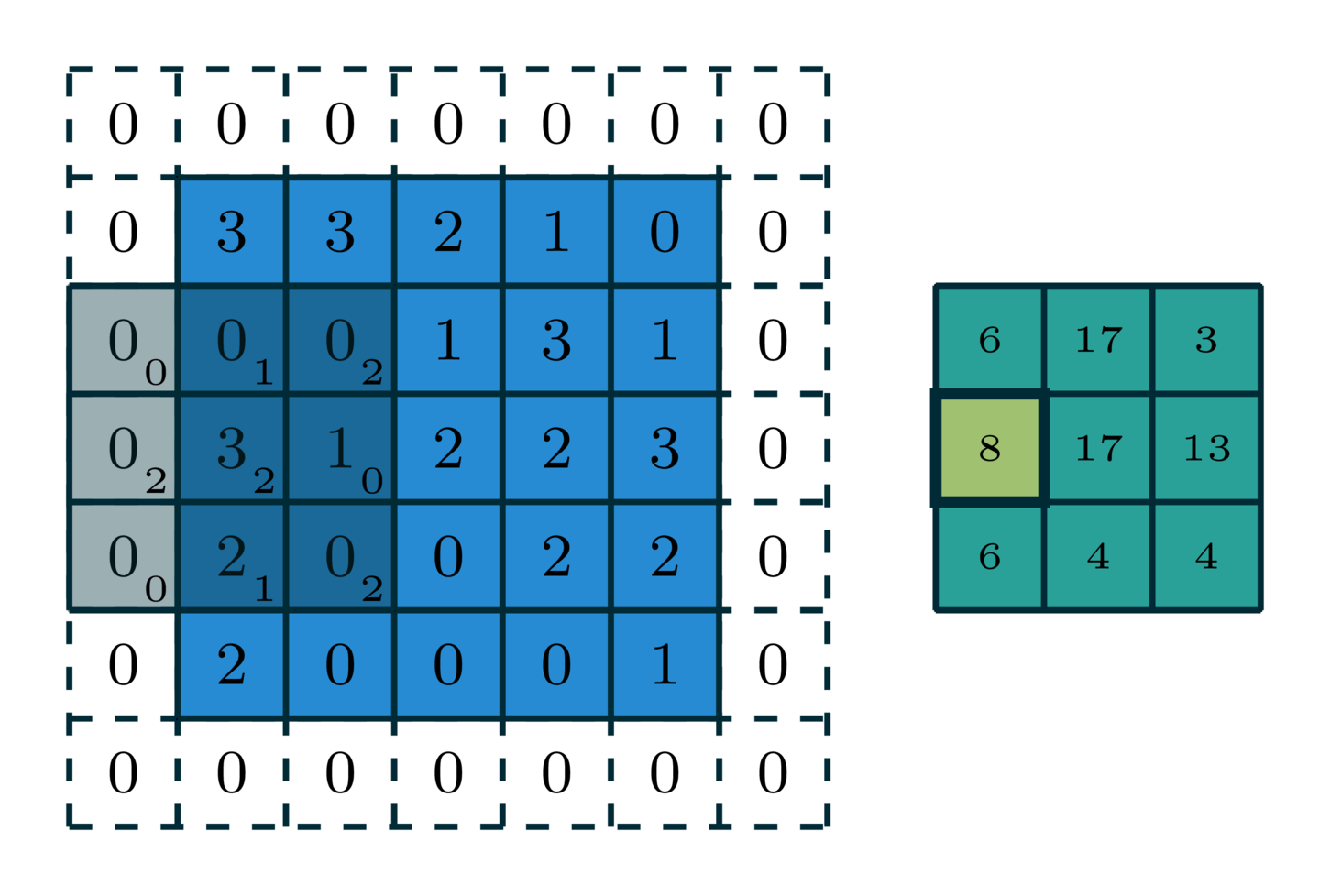
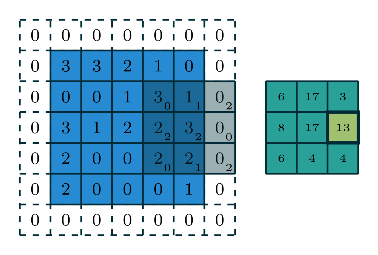
[image edited from vdumoulin]
convolved output
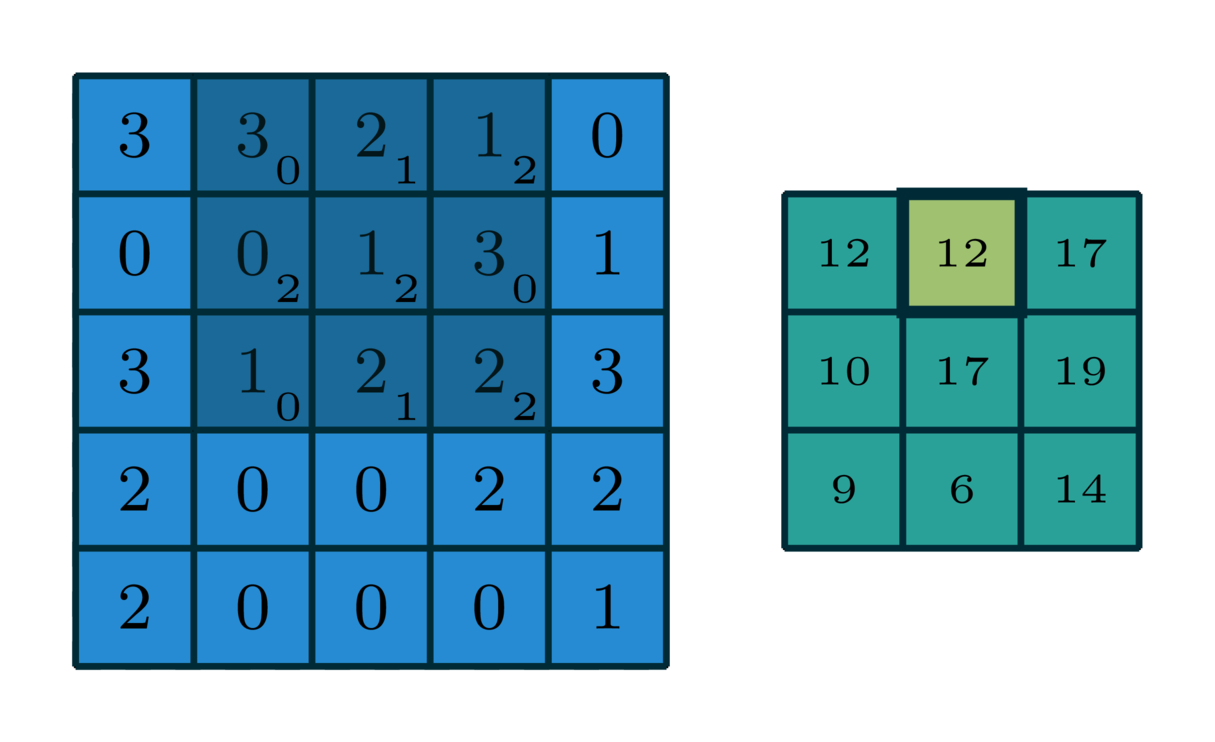
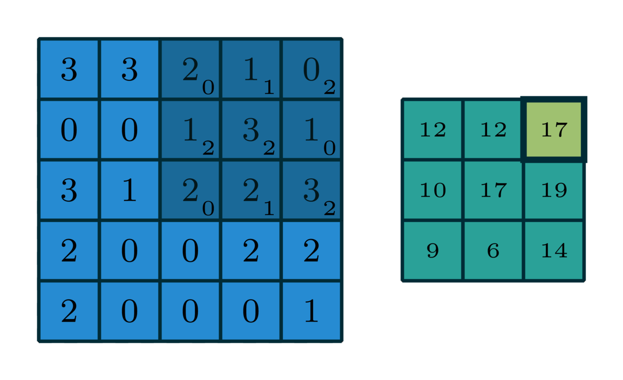
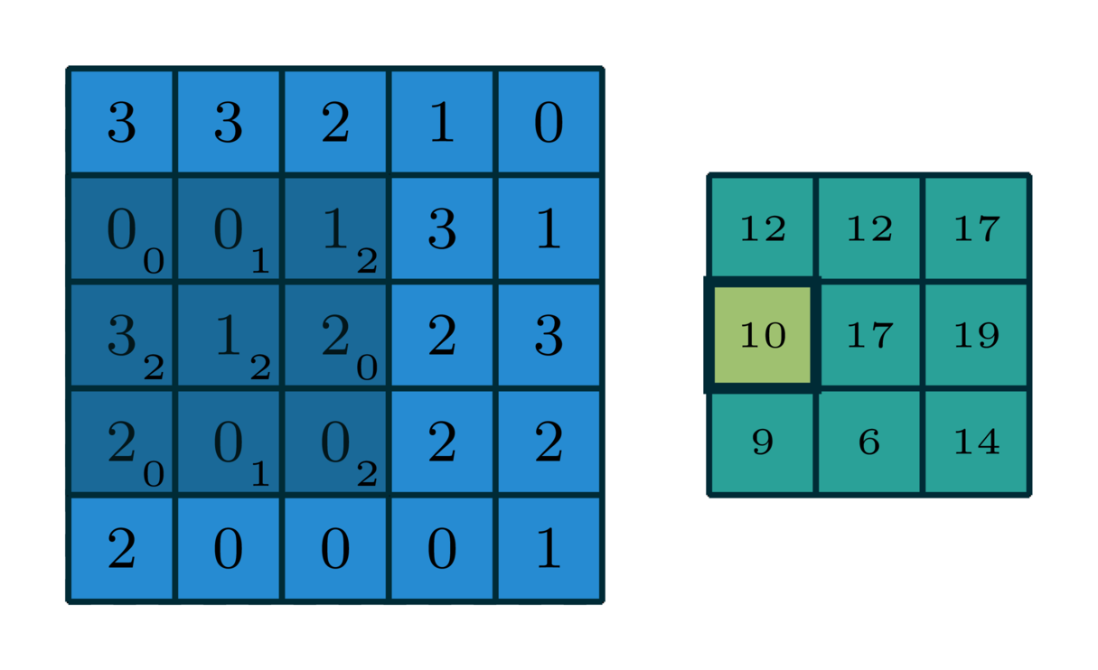
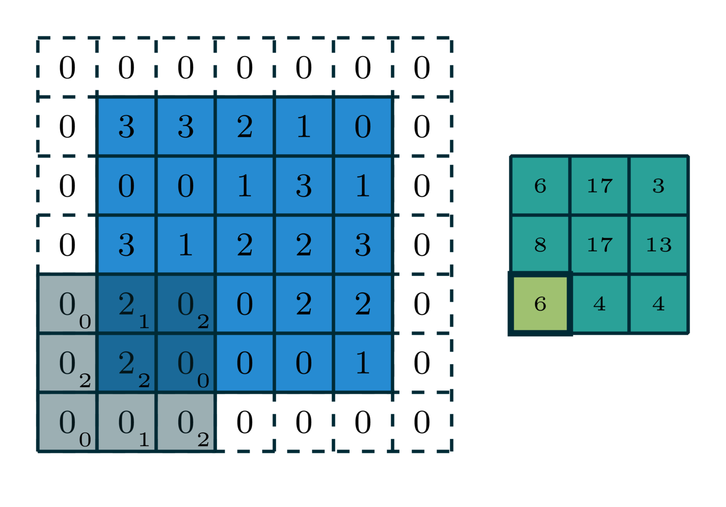
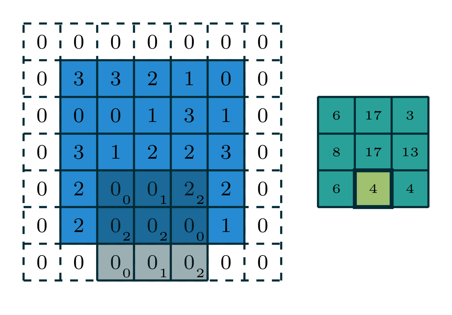
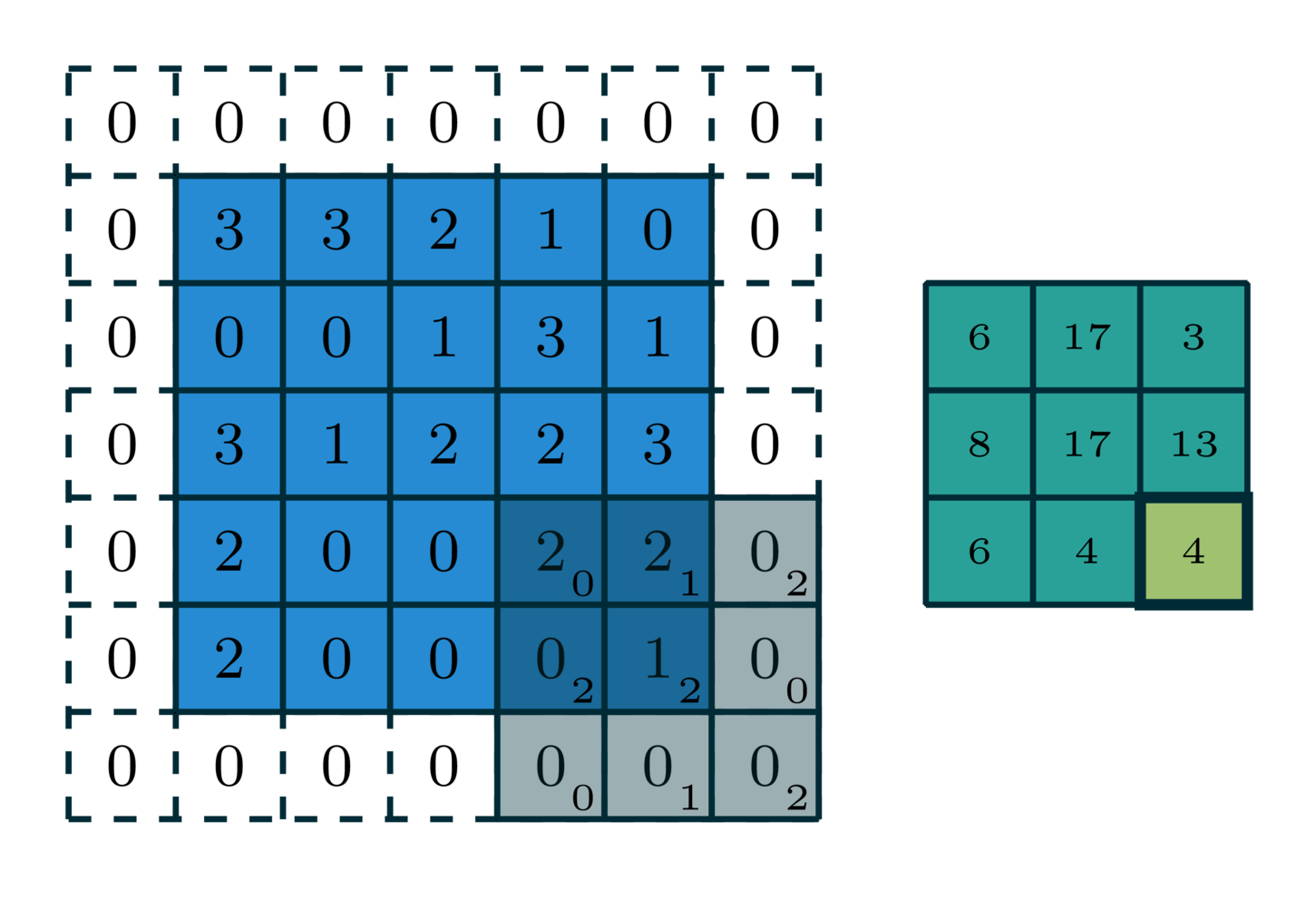
example: 2-dimensional convolution
[image edited from vdumoulin]
[image edited from vdumoulin]
stride of 2
input
filter
output
[image edited from vdumoulin]
[image edited from vdumoulin]
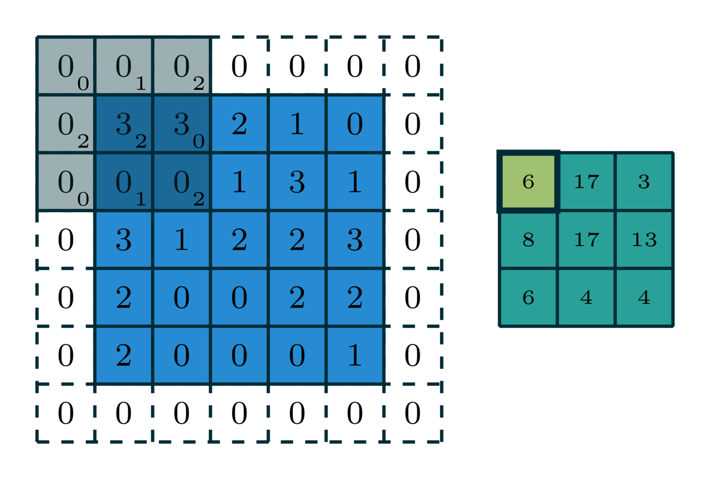
stride of 2, with padding of size 1
input
filter
output
[image edited from vdumoulin]

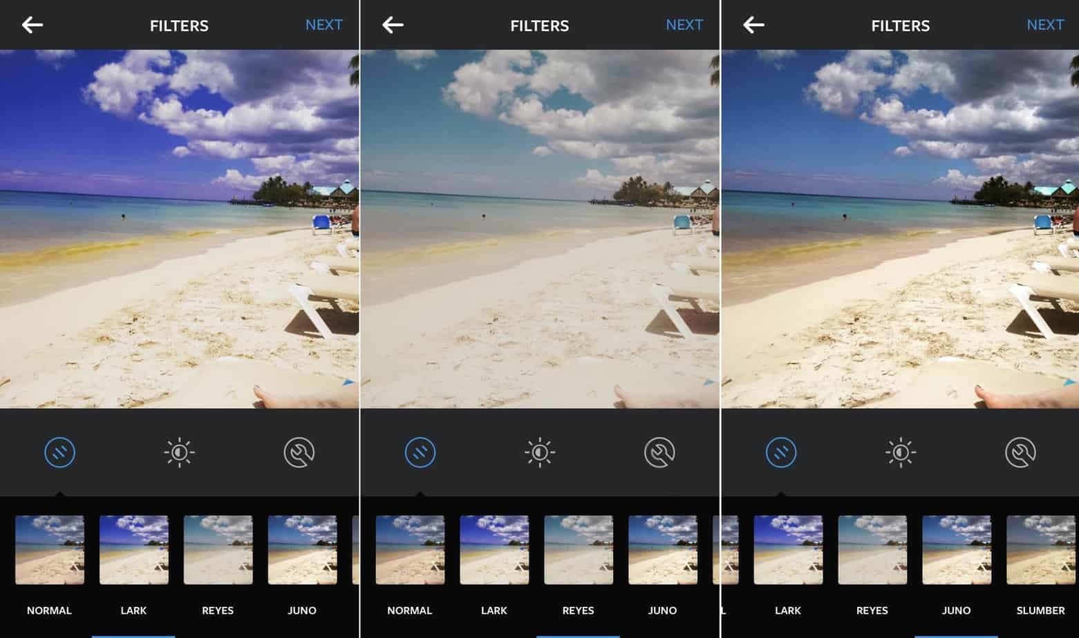
quick summary: hyperparameters for 1d convolution
- Zero-padding
- Filter size (e.g. we saw these two in 1-d)
- Stride
(e.g. stride of 2)
0
0
0
0
0
0
0
0
0
0
0
0
0
0
0
0
0
0
1
1
0
0
1
1
1
1
0
0
1
1
0
0
1
1
1
1
0
0
0
0
0
0
0
0
0
0
1
1
0
0
1
1
1
1
0
0
1
1
0
0
1
1
1
1
0
0
0
0
0
0
0
0
1
these weights are what CNN learn eventually
-1
1
0
0
0
0
1
1
1
1
0
0
0
0
1
1
1
1
1
1
1
1
quick summary: hyperparameters for 2d convolution
[video credit Lena Voita]
- Look locally (sparse connections)
- Parameter sharing
- Template matching
- Translational equivariance
quick summary: convolution interpretation
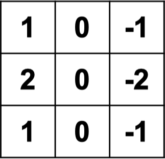
hand-designed filters (e.g. Sobel)
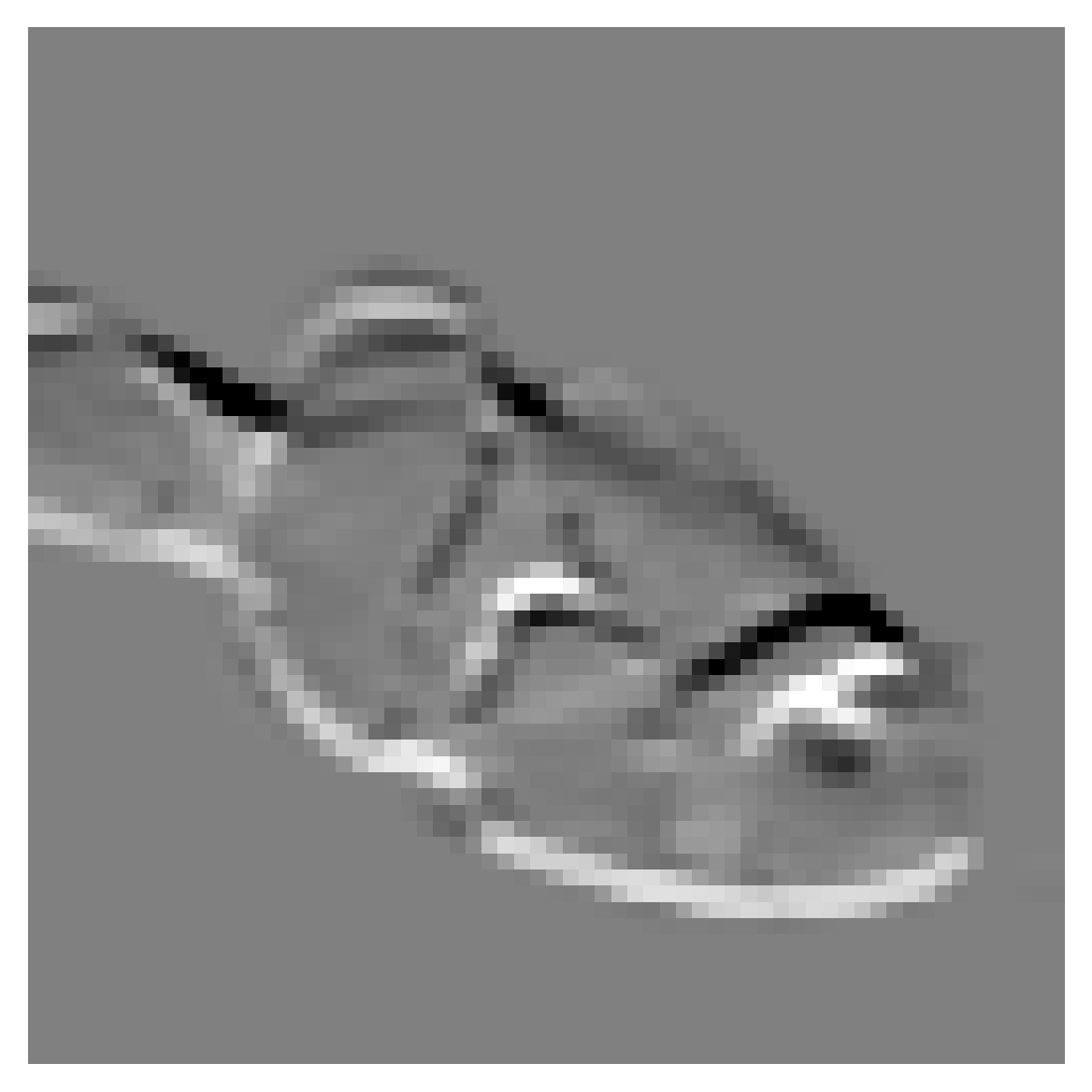
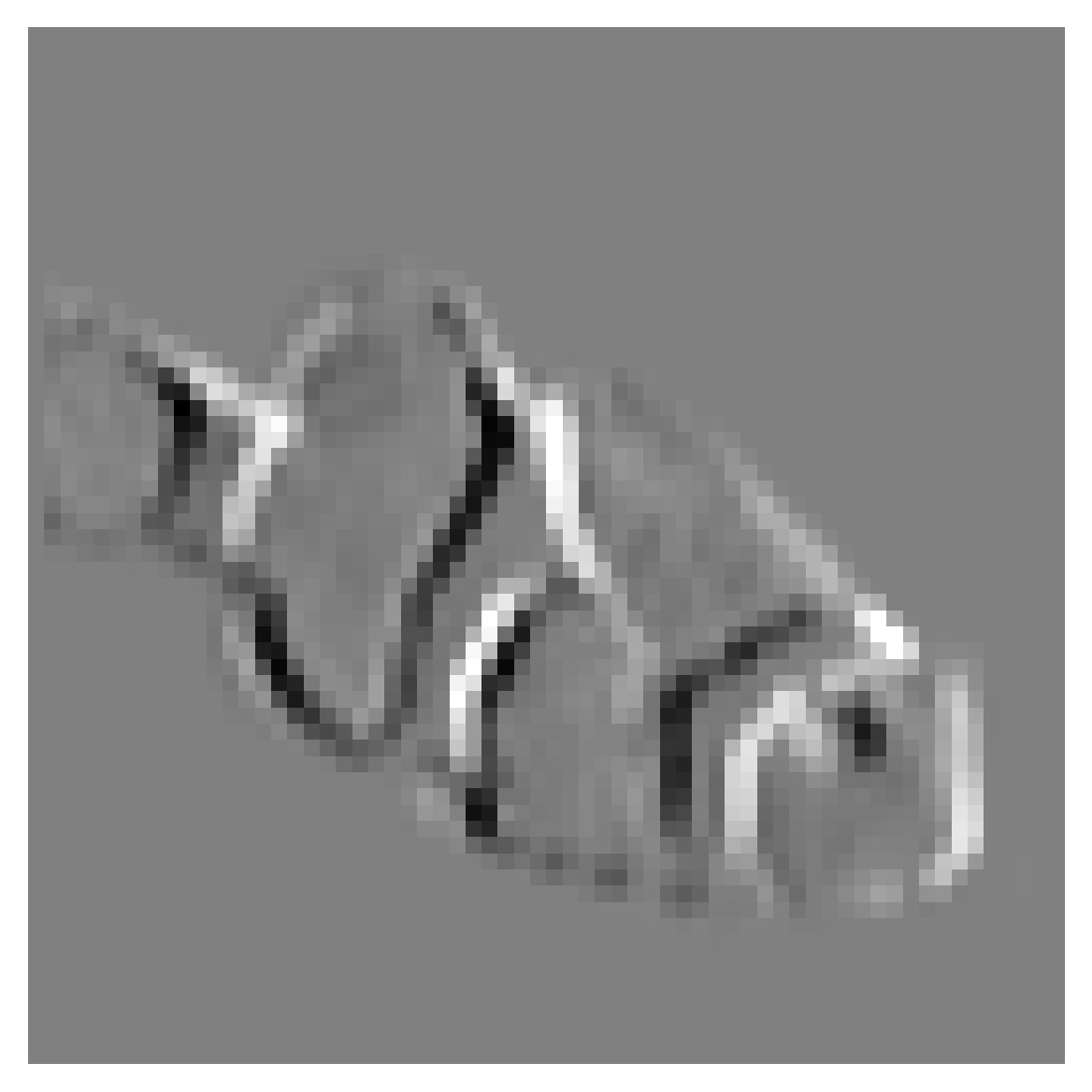
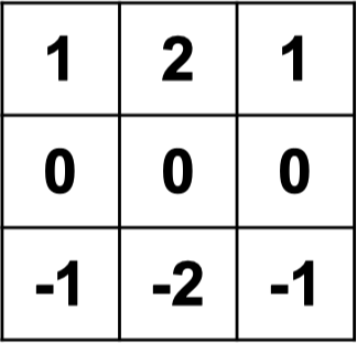
filter 1
filter 2
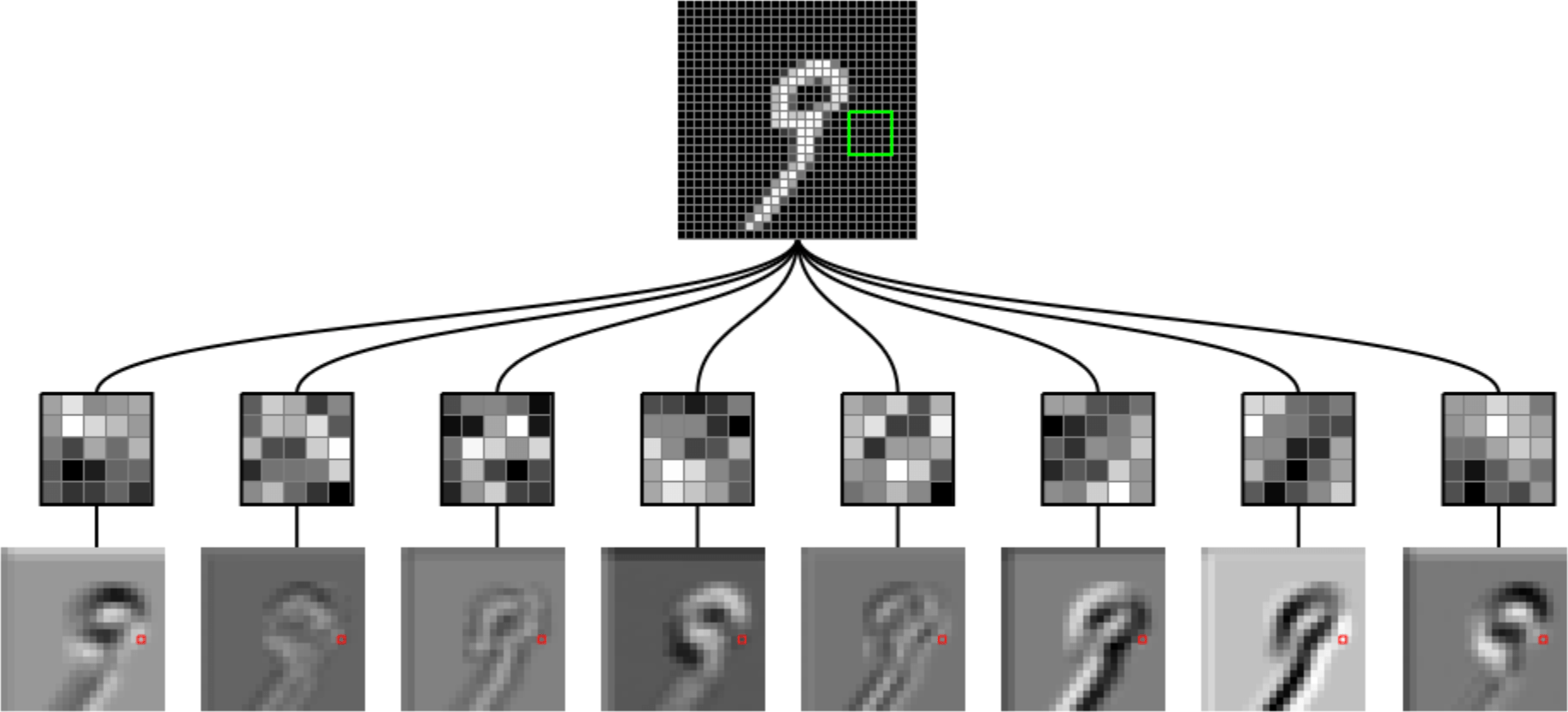
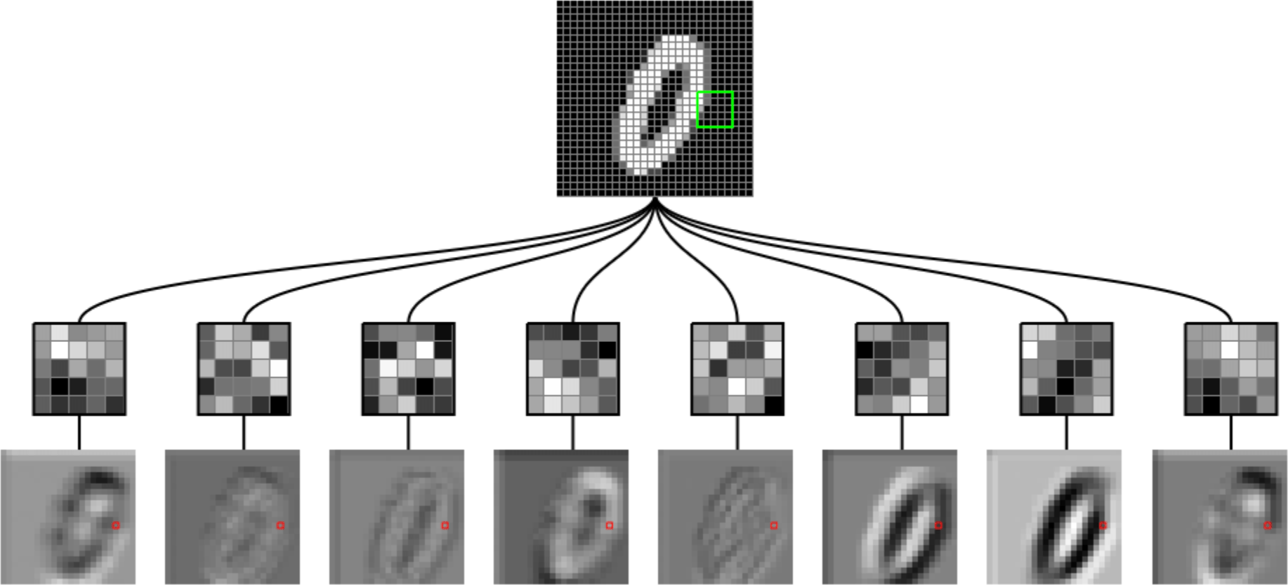
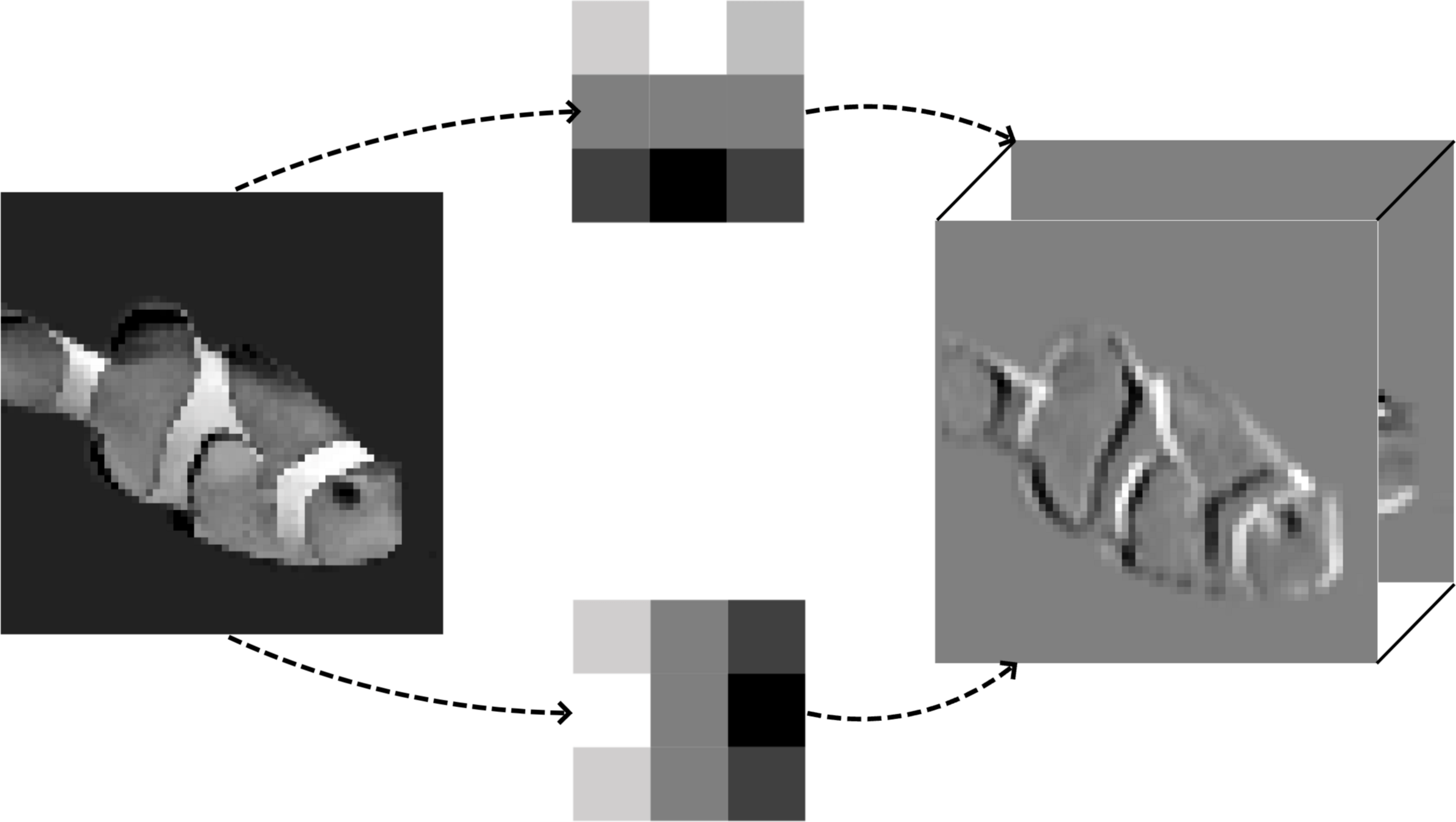
learned filters detect many patterns
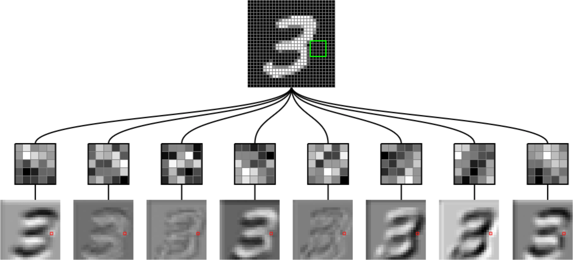
input
filters
conv'd output
Outline
- Vision problem structure
- Convolution
- 1-dimensional and 2-dimensional convolution
- 3-dimensional tensors
- Max pooling
- (Case studies)
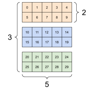
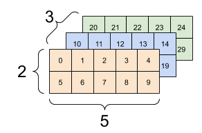
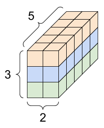
A tender intro to tensor:


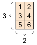
[image credit: tensorflow]
red
green
blue
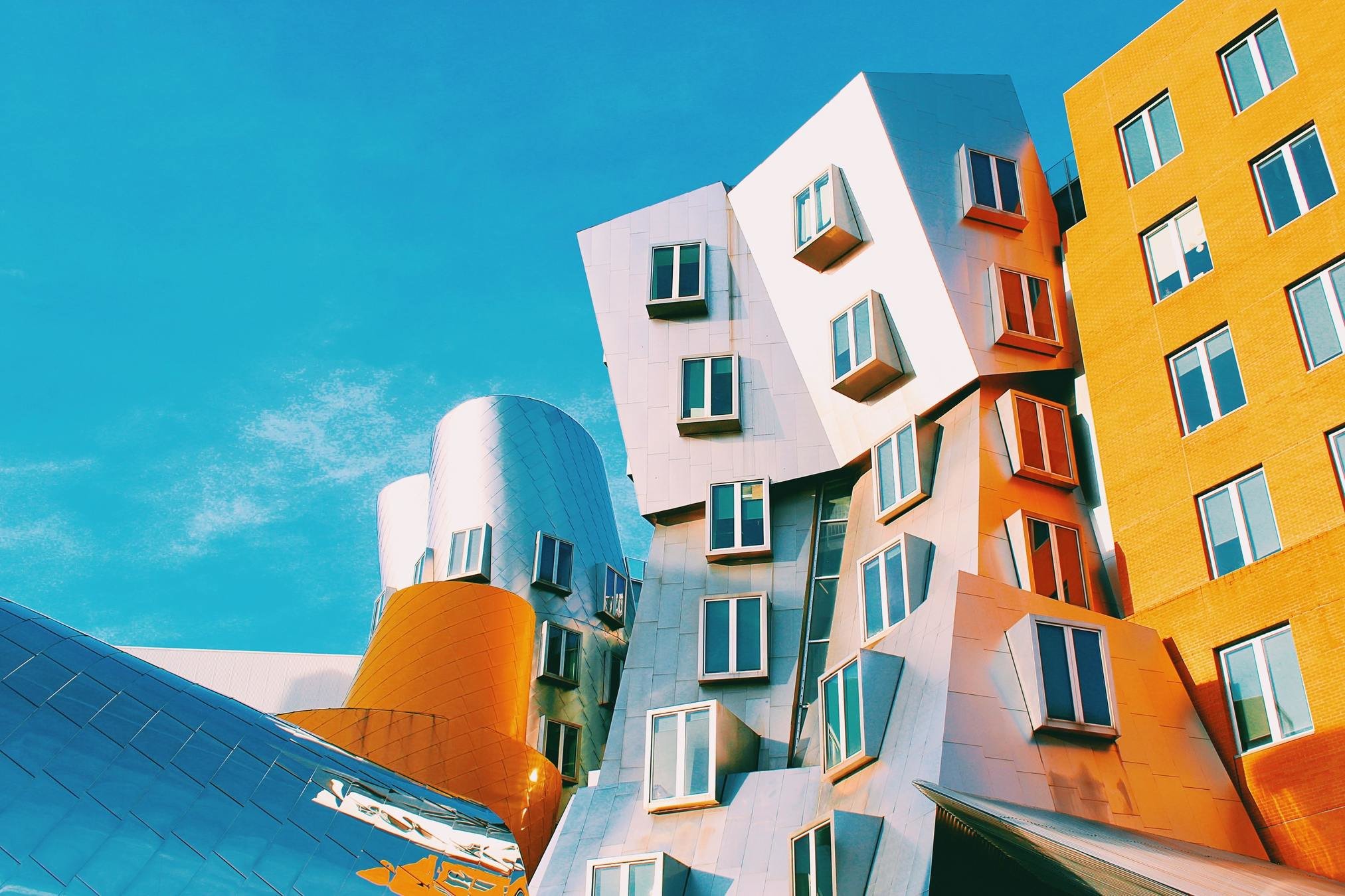
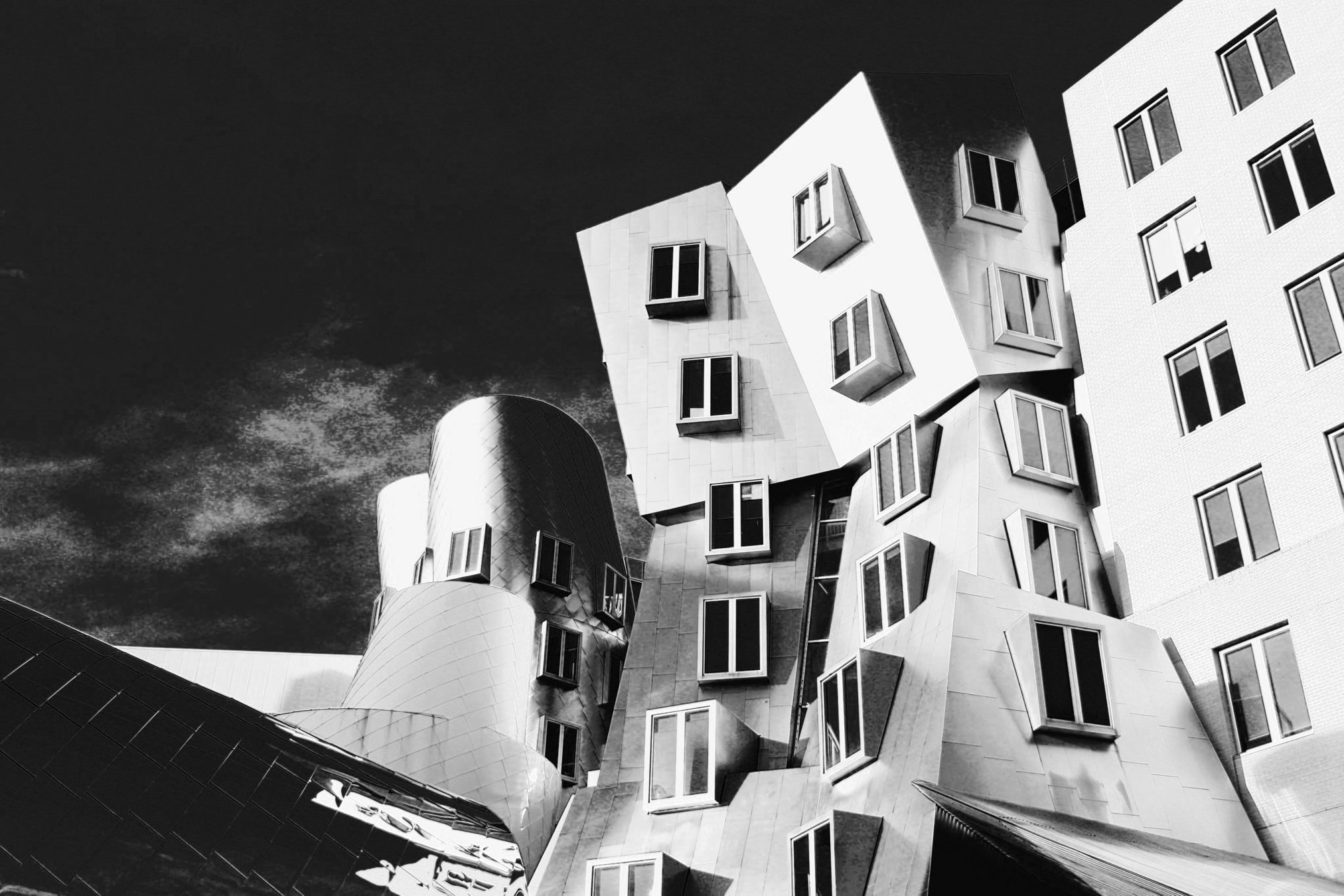
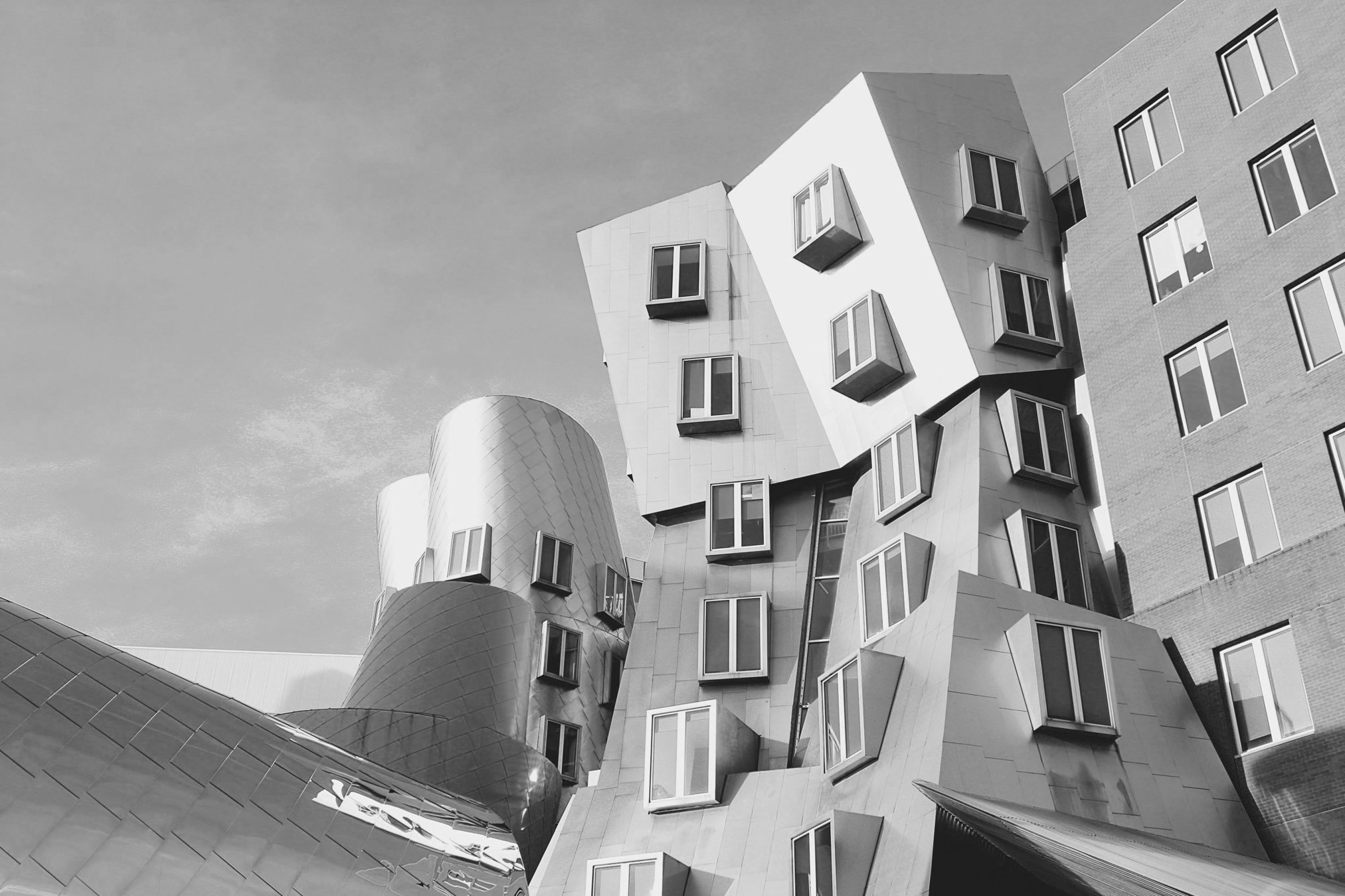
color images and channels
each channel is a complete but independent view of the same scene
like when we think of weather:
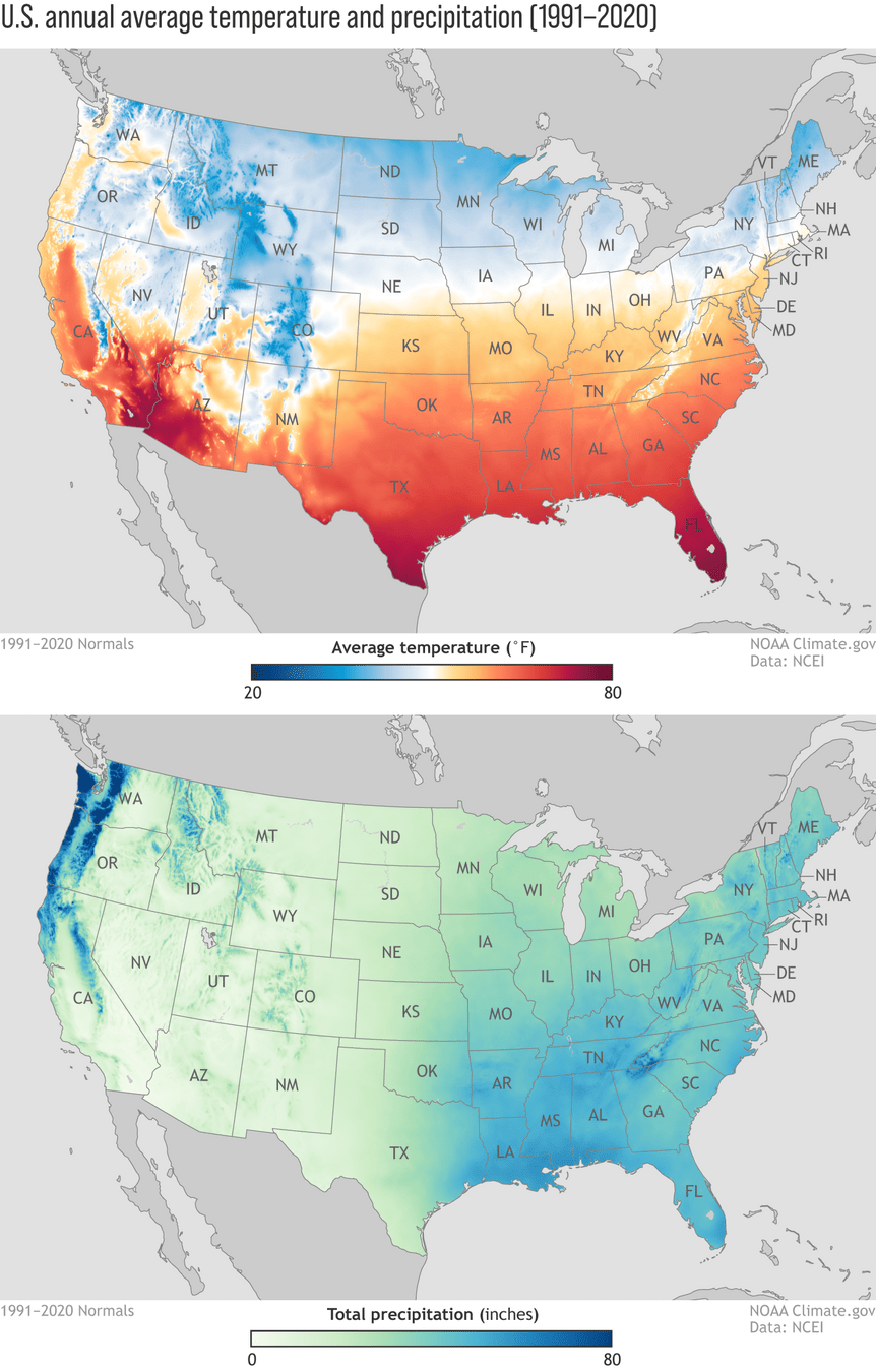
so channels are often referred to as feature maps
image channels
image width
image
height
3d tensors from color channels
filter 1
filter 2
3d tensors from multiple filters
filter 1
filter 2
channels
\dots
3d tensors from multiple filters
2. multiple filters → multiple channels
channels
width
height
channels
1. color input
where do channels come from?
Why we don't typically do 3d convolution
slide along →
slide along ↓
slide along ↗
Convolution shares weights across shifted positions
shifting makes sense spatially (a cat can be anywhere)
but not across channels (red ≠ shifted green)
3D conv is used when the third axis is spatial/temporal (MRI, video)
width
height
- 2d convolution, 2d output
channels
\Bigg\{
d
| ... | ||||
| ... | ||||
| ... | ||||
| ... |
- 3d tensor input, channel \(d\)
- 3d tensor filter, channel \(d\)
output
full-depth 2D convolution
| ... | ||
| ... | ||
| ... | ... | ... |
| ... | ||
| ... | ||
| ... | ... | ... |
| ... | ||
| ... | ||
| ... | ... | ... |
\dots
\dots
input tensor
multiple filters
multiple output matrices
| ... |
| ... |
input tensor
\(k\) filters
output tensor
\dots
\dots
| ... | ||
| ... | ||
| ... | ... | ... |
\Bigg\{
d
\Bigg\{
d
\left\{
\begin{array}{l}
\\
\\
\\
\end{array}
\right.
k
\left\{
\begin{array}{l}
\\
\\
\\
\\
\\
\\
\\
\\
\end{array}
\right.
k
2. the use of multiple filters
1. color input
Every convolutional layer works with 3d tensors:
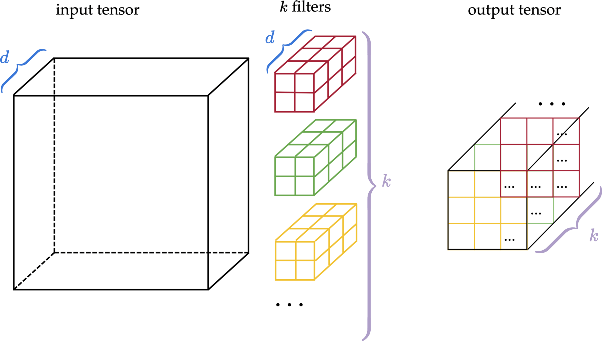
in doing 2d convolution
Outline
- Vision problem structure
- Convolution
- 1-dimensional and 2-dimensional convolution
- 3-dimensional tensors
- Max pooling
- (Case studies)
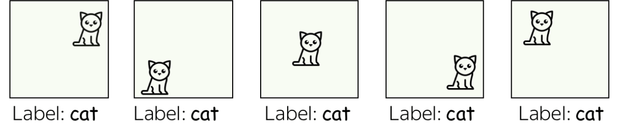
| ✅ | ||||
|---|---|---|---|---|
| ✅ | ||||
| ✅ | ||||
| ✅ | ||||
| ✅ | ||||
|---|---|---|---|---|
cat moves, detection moves
convolution helps detect pattern, but ...
convolution
max pooling
slide w. stride
slide w. stride
no learnable parameter
learnable filter weights
ReLU
summarizes strongest response
detects pattern
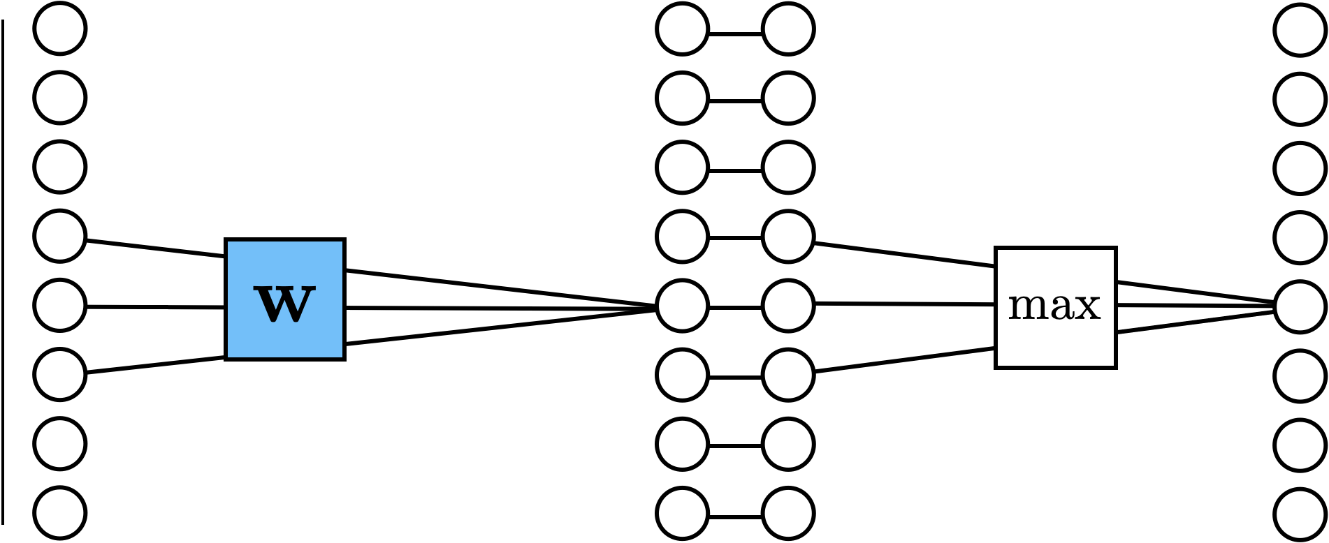
1d max pooling
2d max pooling
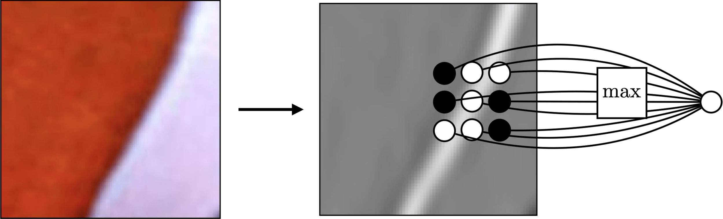
[image credit Philip Isola]
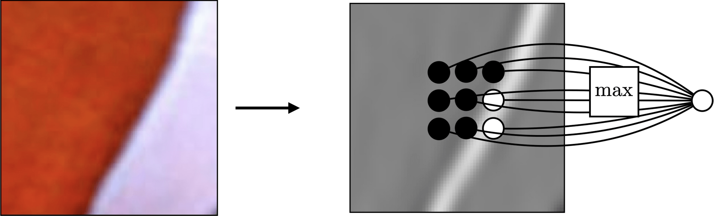
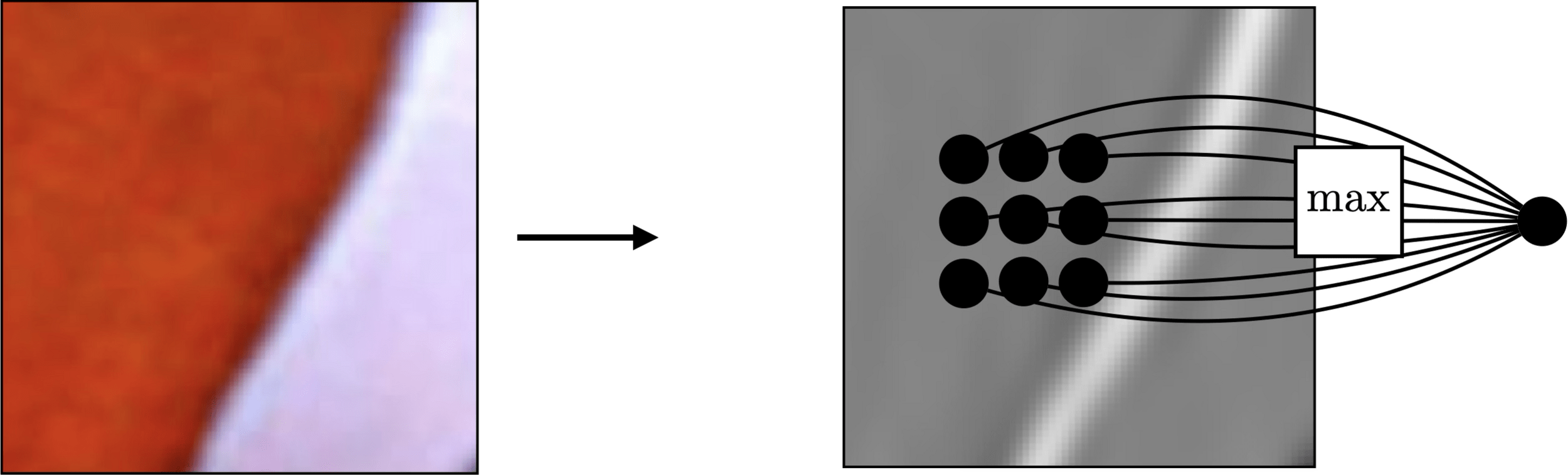
large response regardless of exact position of edge
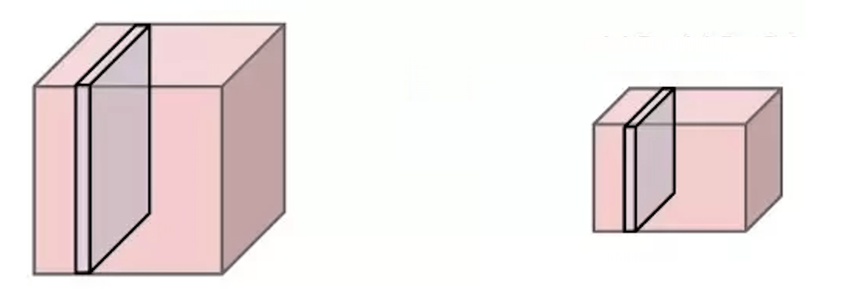
Pooling across spatial locations achieves invariance w.r.t. small translations:
Pooling across spatial locations achieves invariance w.r.t. small translations:
\Bigg\{
\begin{array}{l}
\\
\\
\\
\\
\\
\end{array}
\Bigg.
\Bigg\{
\begin{array}{l}
\\
\\
\\
\\
\\
\end{array}
\Bigg.
\{
channels
channels
height
width
\{
width
height
\left\{
\begin{array}{l}
\\
\\
\end{array}
\right.
\Bigg\{
\begin{array}{l}
\\
\\
\\
\\
\\
\end{array}
\Bigg.
so the channel dimension remains unchanged
pooling
applied independently across all channels
Outline
- Vision problem structure
- Convolution
- 1-dimensional and 2-dimensional convolution
- 3-dimensional tensors
- Max pooling
- (Case studies)
[image credit Philip Isola]
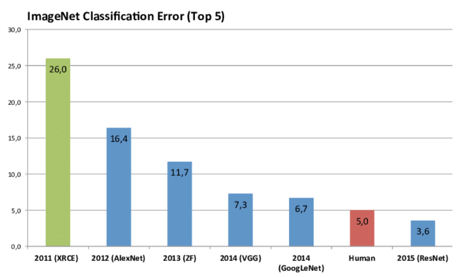
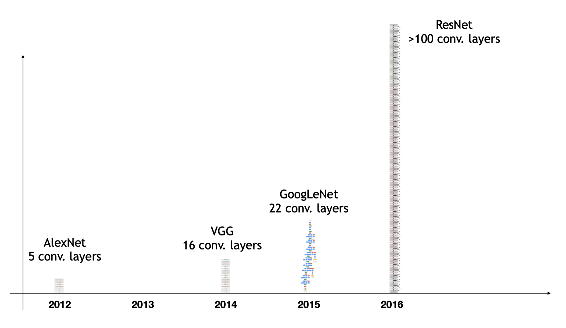
CNN renaissance
filter weights
fully-connected neuron weights
\nabla \mathcal{L}
\mathcal{L}
label
image
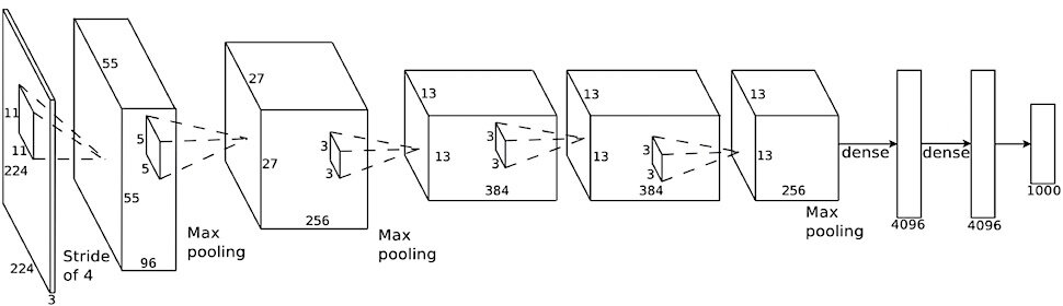
[all max pooling are 3×3 filter, stride 2; pooled outputs not explicitly shown on diagram: 27×27×96, 13×13×256, 6×6×256]
[image credit Philip Isola]
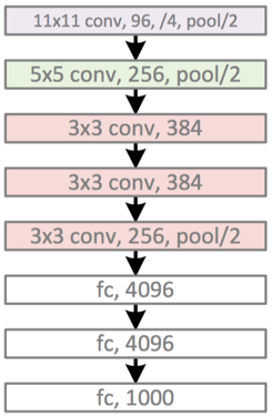
AlexNet '12
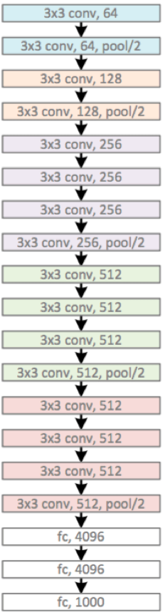
VGG '14
“Very Deep Convolutional Networks for Large-Scale Image Recognition”, Simonyan & Zisserman. ICLR 2015
[image credit Philip Isola and Kaiming He]
VGG '14
Main developments:
- small convolutional filters: only 3x3
- increased depth: about 16 or 19 layers of the same modules
VGG '14
[He et al: Deep Residual Learning for Image Recognition, CVPR 2016]
[image credit Philip Isola and Kaiming He]
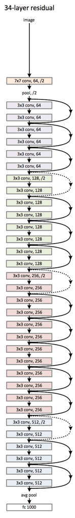

ResNet '16
Main developments:
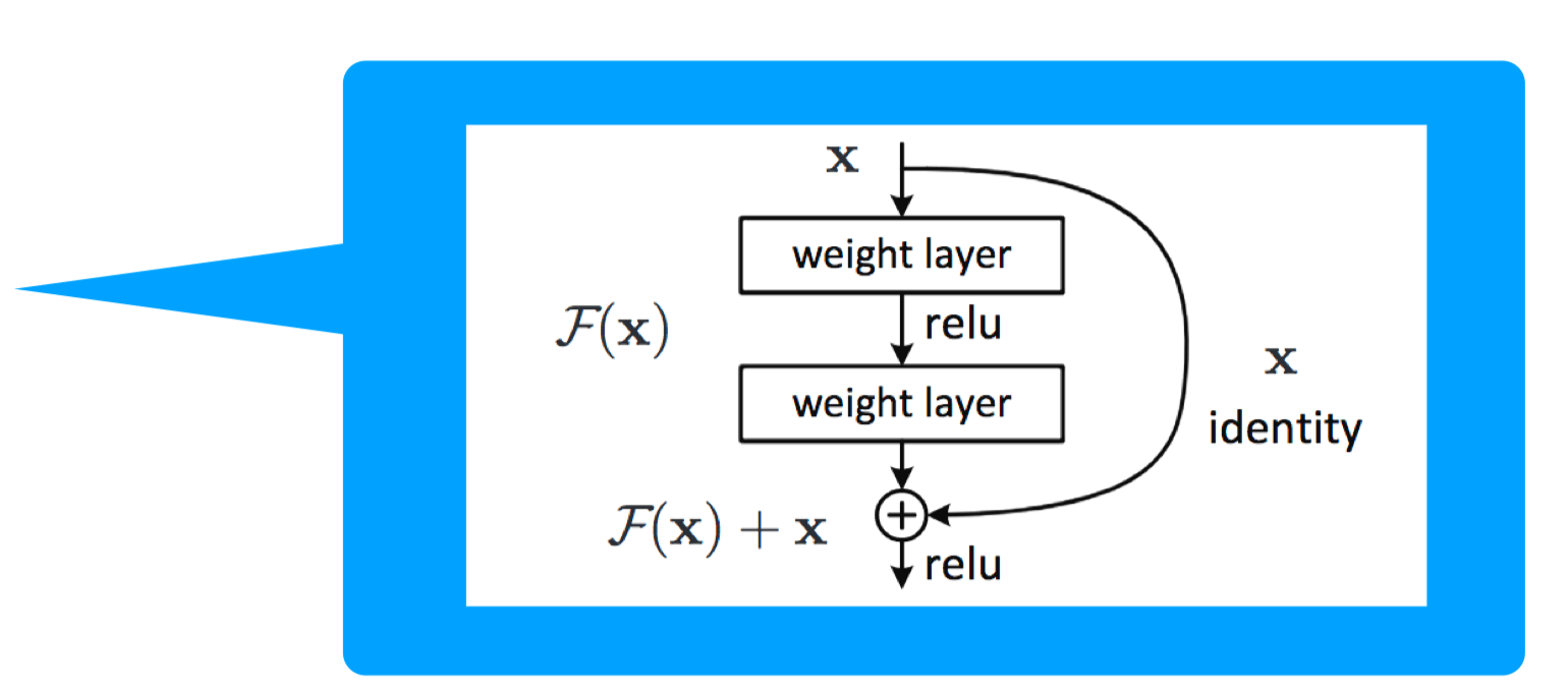
- Residual block -- gradients can propagate faster (via the identity mapping)
- increased depth: > 100 layers
Summary
Even though NNs are universal approximators, matching the architecture to problem structure — visual hierarchy, locality, translational invariance — improves generalization and efficiency.
Convolution slides a small learned filter across the input, detecting local patterns with shared weights — sparse and efficient.
Max pooling summarizes spatial information: "did a pattern occur?" rather than "where exactly?"
Filter weights are learned end-to-end; convolutional layers extract features, fully connected layers classify.
[video edited from 3b1b]
[video edited from 3b1b]
[video edited from 3b1b]
[video edited from 3b1b]
\underbrace{\hspace{6.5cm}}
\frac{\partial Z^2}{\partial A^{1}}
\frac{\partial A^1}{\partial Z^{1}}
\frac{\partial Z^1}{\partial W^{1}}
x
\(\dots\)
y
f^1
\begin{aligned}
& W^1 \\
\end{aligned}
\begin{aligned}
& W^2 \\
\end{aligned}
\begin{aligned}
& W^L \\
\end{aligned}
f^L
\mathcal{L}(g,y)
g
Z^L
A^2
Z^2
A^1
Z^1
\frac{\partial \mathcal{L}(g,y)}{\partial g}
\frac{\partial g}{\partial Z^{L}}
\frac{\partial Z^3}{\partial A^{2}}\frac{\partial A^4}{\partial Z^{3}} \dots \frac{\partial Z^L}{\partial A^{L-1}}
\frac{\partial A^2}{\partial Z^{2}}
\frac{\partial \mathcal{L}(g,y)}{\partial Z^2}
\underbrace{\hspace{4cm}}
\frac{\partial \mathcal{L}(g,y)}{\partial W^1}
Now
f^2
\frac{\partial \mathcal{L}(g,y)}{\partial W^1}
how to find
?
\frac{\partial \mathcal{L}(g,y)}{\partial W^1}
x
\(\dots\)
y
f^1
\begin{aligned}
& W^1 \\
\end{aligned}
\begin{aligned}
& W^2 \\
\end{aligned}
\begin{aligned}
& W^L \\
\end{aligned}
f^L
\mathcal{L}(g,y)
g
Z^L
A^2
Z^2
A^1
Z^1
\frac{\partial \mathcal{L}(g,y)}{\partial g}
\frac{\partial g}{\partial Z^{L}}
\frac{\partial Z^3}{\partial A^{2}}\frac{\partial A^4}{\partial Z^{3}} \dots \frac{\partial Z^L}{\partial A^{L-1}}
\frac{\partial A^2}{\partial Z^{2}}
\frac{\partial \mathcal{L}(g,y)}{\partial Z^2}
\frac{\partial Z^2}{\partial W^{2}}
\underbrace{\hspace{4.7cm}}
\frac{\partial \mathcal{L}(g,y)}{\partial W^2}
how to find
?
Previously, we found
f^2
\underbrace{\hspace{4cm}}
x
\(\dots\)
y
f^1
\begin{aligned}
& W^1 \\
\end{aligned}
\begin{aligned}
& W^2 \\
\end{aligned}
\begin{aligned}
& W^L \\
\end{aligned}
f^2
f^L
\mathcal{L}(g,y)
g
\underbrace{\hspace{4.7cm}}
Z^L
A^2
Z^2
A^1
Z^1
\frac{\partial \mathcal{L}(g,y)}{\partial W^2}
\frac{\partial \mathcal{L}(g,y)}{\partial g}
\frac{\partial g}{\partial Z^{L}}
\frac{\partial Z^3}{\partial A^{2}}\frac{\partial A^4}{\partial Z^{3}} \dots \frac{\partial Z^L}{\partial A^{L-1}}
\frac{\partial A^2}{\partial Z^{2}}
\frac{\partial Z^2}{\partial W^{2}}
\frac{\partial \mathcal{L}(g,y)}{\partial Z^2}
\underbrace{\hspace{4cm}}
\frac{\partial \mathcal{L}(g,y)}{\partial W^2}
?
suppose we sampled a particular \((x,y),\) how to find
- can choose filter size
- typically choose to have no padding
- typically a stride >1
- reduces spatial dimension
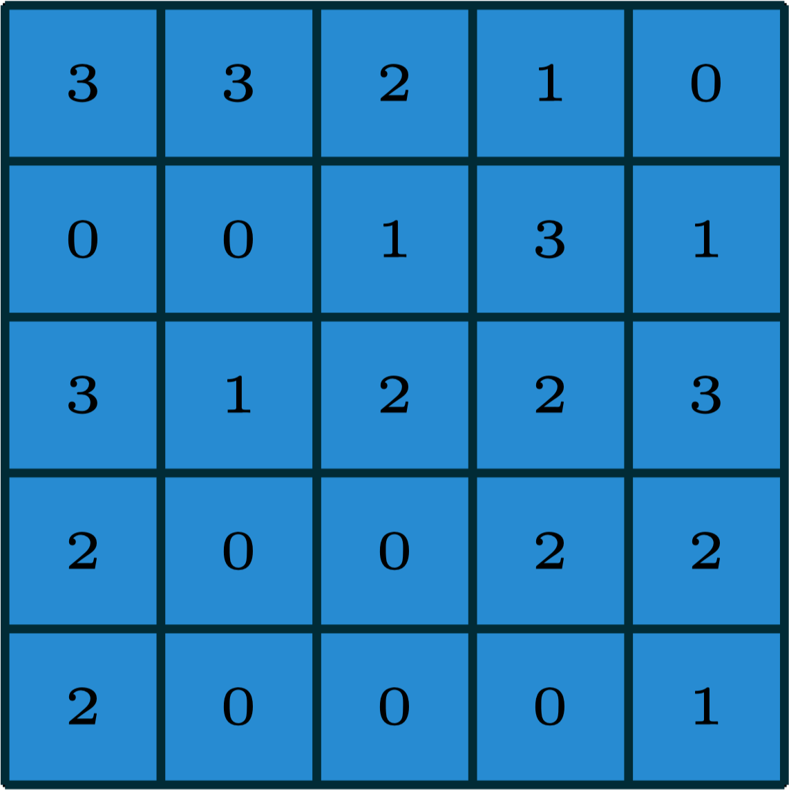
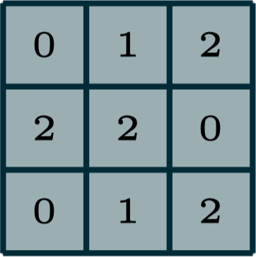
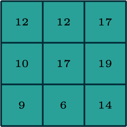
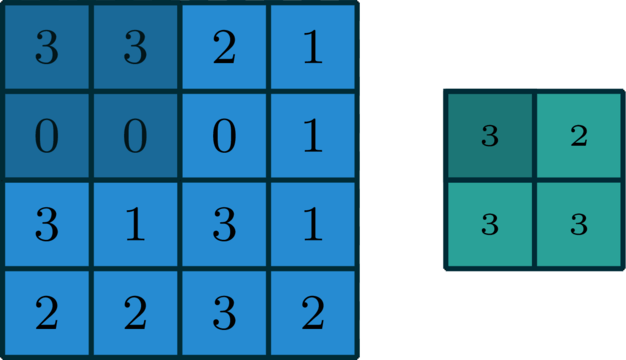
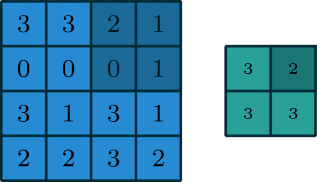
2-dimensional max pooling (example)
| ... | ||||
| ... | ||||
| ... | ||||
input tensor
one filter
2d output
- 3d tensor input, channel \(d\)
- 3d tensor filter, channel \(d\)
- 2d tensor (matrix) output
6.390 IntroML (Spring26) - Lecture 7 Convolutional Neural Networks
By Shen Shen


