Strategies: Heat Equation
Parallel Algorithms
David Mayerich
Scalable Tissue Imaging and Modeling (STIM) Laboratory
Department of Electrical and Computer Engineering
Cullen College of Engineering
University of Houston
David Mayerich
STIM Laboratory, University of Houston

2D Heat Equation
-
Constants: thermal conductivity \(k\), density \(\rho\), and heat capacity \(c\)
-
\(T\) is the temperature measured at point \((x,y)\) at time \(t\)
-
Laplace operator (Laplacian):
David Mayerich
STIM Laboratory, University of Houston
\frac{\partial T}{\partial t} =
\frac{k}{\rho c}
\left(
\frac{\partial^2 T}{\partial x^2}
+
\frac{\partial^2 T}{\partial y^2}
\right)
=
\frac{k}{\rho c}\nabla^2 T
\nabla^2 = \sum_i \frac{\partial}{\partial x_i}

change in temperature over time
material properties
heat flow along both directions
Discretization
-
Track the discrete temperature on a grid:
David Mayerich
STIM Laboratory, University of Houston
-
Each discrete spatial location \((x_i,y_j)\) stores the temperature at time \(t_n\)
-
Spacing between grid points is consistent (but doesn't have to be):
\(\Delta_x = x_{i+1}-x_i \quad\quad \Delta_y = y_{j+1}-y_j\) -
We update this grid to calculate the temperature at each time step:
\(\Delta_t = t_{n+1}-t_n\)-
Step values are specified by the user
-
Related to actual spatial locations and time points, for example:
\(x_i = x_0 + i\cdot \Delta_x\)
-
T_{i,j}^n = T[i,j,n]=T(x_i,y_j,t_n)
T(x_i,y_j, t_n)
T(x_{i+1},y_{j+2}, t_n)
\Delta_x
\Delta_y
Finite Difference Calculus
-
Start from a first-order Taylor series:
David Mayerich
STIM Laboratory, University of Houston
f(x)\approx f(c)+f'(c)(x-c) + O\left[(x-c)^2\right]
-
Given two known points \(c=x_i\) and \(x=x_{i+1}=x_i + x_\Delta\):
f(x_{i+1}) \approx f(x_i)+f'(x_i)(x_{i+1}-x_i) + O\left[(x_{i+1}-x_i)^2\right]
f(x_{i+1}) \approx f(x_i)+f'(x_i)(x_\Delta) + O\left(x_\Delta^2\right)
-
Solve for \(f'(x)\):
f'(x_i) \approx \frac{f(x_{i+1})-f(x_i) + O\left(x_\Delta^2 \right)}{x_\Delta}
-
Note that the order in the error term is reduced:
f'(x_i) \approx \frac{f(x_{i+1})-f(x_i)}{x_\Delta} + O\left(x_\Delta\right)
Finite Difference Calculus
-
Finite difference methods are used to approximate a partial derivative from samples of a function:
David Mayerich
STIM Laboratory, University of Houston
-
Given these approximations for the spatial partial derivatives, we want to compute \(T\) at \(t_{n+1}\) based on the diffusion equation:
\frac{\partial T}{\partial t} =
\alpha
\left(
\frac{\partial^2 T}{\partial x^2}
+
\frac{\partial^2 T}{\partial y^2}
\right)
\frac{\partial f}{\partial x}\approx
\frac{f(x_{i+1}) - f(x_{i-1})}{2\Delta_x}
\approx
\frac{f(x_{i+1}) - f(x_{i})}{\Delta_x}
\approx
\frac{f(x_{i}) - f(x_{i-1})}{\Delta_x}
O(\Delta_x^2)
O(\Delta_x)
O(\Delta_x)
-
Approximating the second derivative:
\frac{\partial^2 f}{\partial x^2}\approx
\frac{f(x_{i+1}) - 2f(x_i) + f(x_{i-1})}{\Delta_x^2}
\Delta_t
T^n_{i,j}=T(x_i,y_j, t_n)
T^{n+1}_{i,j} = T(x_i,y_j, t_{n+1})
Explicit Method
-
Given the temperature \(T^n_{i,j}\) at \(t_n\), we approximate the future temperature \(T^{n+1}_{i,j}\) at \(t_{n+1}\) using the forward finite difference:
David Mayerich
STIM Laboratory, University of Houston
-
Using the same finite difference methods, we can approximate the two spatial derivatives:
\frac{\partial^2 T}{\partial x^2}\approx
\frac{T^n_{i+1, j} - 2T^n_{i,j} + T^n_{i-1,j}}{\Delta^2_x}
\frac{\partial T}{\partial t} =
\alpha
\left(
\frac{\partial^2 T}{\partial x^2}
+
\frac{\partial^2 T}{\partial y^2}
\right)
\frac{\partial T}{\partial t} \approx
\frac{T^{n+1} - T^n}{\Delta_t}
T^{n+1}
\approx
T^n + \Delta_t \frac{\partial T}{\partial t}
by solving for \(T^{n+1}\):
which depends on the partial differential equation we already know:
\frac{\partial^2 T}{\partial y^2}\approx
\frac{T^n_{i, j+1} - 2T^n_{i,j} + T^n_{i,j-1}}{\Delta^2_y}
-
Assuming \(h=\Delta_x = \Delta_y\) and collecting terms, we have:
\frac{\partial T}{\partial t}
\approx
\frac{\alpha}{h^2}
\left(
T^n_{i+1,j} + T^n_{i-1,j} + T^n_{i,j+1} + T^n_{i,j-1} - 4T^n_{i,j}
\right)
Algorithm: Explicit Euler Method
Euler's Method: solves a PDE using a first-order (Taylor Series) approximation
Given the value of \(T^n_{i,j}=T(x_i, y_j, t_n)\)
Approximate the PDE at every point:
David Mayerich
STIM Laboratory, University of Houston
\frac{\partial T_{i,j}^n}{\partial t}
\approx
\frac{\alpha}{h^2}
\left(
T^n_{i+1,j}+T^n_{i-1,j}+T^n_{i,j+1}+T^n_{i,j-1}-4T^n_{i,j}
\right)
-
Update every point to the next time step:
T^{n+1}_{i,j} \leftarrow
T^n_{i,j}+\Delta_t \frac{\partial T^n_{i,j}}{\partial t}
T^n_{i,j}
\Delta_x
\Delta_y
\Delta_t
T^{n+1}_{i,j}
Simulation Error
-
Finite difference methods are based on Taylor series:
\(f(x)=f(c)+f'(c)(x-c)+O(\Delta_x)\)-
where \(c=x_i\) and \(x=x_{i+1}\):
\(f(x_{i+1})=f(x)+f'(x_i)\Delta_x + O(\Delta_x)\) -
solve for the derivative:
\(f'(x_i)=\frac{f(x_{i+1}) - f(x)}{\Delta_x} + O(\Delta_x)\)
-
-
Second derivative error:
David Mayerich
STIM Laboratory, University of Houston
-
Error term depends on sample spacing: \(E = O(\Delta_x^2)\)
-
Smaller samples provide better accuracy but increase compute time
-
Stability is based on the Courant-Friedrichs-Lewy (CFL) condition:
Approximation
Error and Stability
f''(x_i)=\frac{
\frac{
f(x_{i+1})-f(x_i)
}{\Delta_x}
-
\frac{f(x_i) - f(x_{i-1})}
{\Delta_x}
}{\Delta_x}
+O(\Delta_x)
f''(x_i)=\frac{
f(x_{i+1})-2f(x_i)+f(x_{i-1})
}
{\Delta_x^2}
+O(\Delta_x^2)
\alpha \Delta_t
\left(
\frac{1}{\Delta_x^2}
+
\frac{1}{\Delta_y^2}
\right)
\leq
\frac{1}{2}
-
Select \(\Delta_x\), \(\Delta_y\), and \(\Delta_t\) to optimize accuracy and minimize compute time
Implementation 1: Follow the Math
David Mayerich
STIM Laboratory, University of Houston
void heat(float* A, float alpha, float h, float dt, int S, float epsilon) {
}
Implementation 1: Follow the Math
David Mayerich
STIM Laboratory, University of Houston
void heat(float* A, float alpha, float h, float dt, int S, float epsilon) {
  float* B = new float[S * S];		// create a new array to store the output
  float c = alpha / (h * h); 		// pre-compute the spatial diffusion term
  while(true) { 					// loop indefinitely
  }
}
Implementation 1: Follow the Math
David Mayerich
STIM Laboratory, University of Houston
void heat(float* A, float alpha, float h, float dt, int S, float epsilon) {
  float* B = new float[S * S];		// create a new array to store the output
  float c = alpha / (h * h); 		// pre-compute the spatial diffusion term
  while(true) { 					// loop indefinitely
    float diff = 0.0f; 				// track how much the simulation result has changed
  }
}
Implementation 1: Follow the Math
David Mayerich
STIM Laboratory, University of Houston
void heat(float* A, float alpha, float h, float dt, int S, float epsilon) {
  float* B = new float[S * S];		// create a new array to store the output
  float c = alpha / (h * h); 		// pre-compute the spatial diffusion term
  while(true) { 					// loop indefinitely
    float diff = 0.0f; 				// track how much the simulation result has changed
    // iterate through each pixel (why y then x?), note boundaries
	for(int j=1; j<S; j++) {
	  for(int i=1; i<S; i++) {

      }
    }

  }
}
Implementation 1: Follow the Math
David Mayerich
STIM Laboratory, University of Houston
void heat(float* A, float alpha, float h, float dt, int S, float epsilon) {
  float* B = new float[S * S];		// create a new array to store the output
  float c = alpha / (h * h); 		// pre-compute the spatial diffusion term
  while(true) { 					// loop indefinitely
    float diff = 0.0f; 				// track how much the simulation result has changed
    // iterate through each pixel (why y then x?), note boundaries
	for(int j=1; j<S; j++) {
	  for(int i=1; i<S; i++) {
        // calculate the partial derivative with respect to time (main calculation)
        dT_dt = c * (A[j*S+i+1] + A[j*S+i-1] + A[(j+1)*S+i] + A[(j-1)*S+i] – 4*A[j*S+i];
	    B[j*S+i] = A[j*S+i] + dt * dT_dt; 			// use explicit integration
		diff += fabs(B[j*S+i] - A[j*S+i]); 			// sum the absolute change
      }
    }

  }
}
Implementation 1: Follow the Math
David Mayerich
STIM Laboratory, University of Houston
void heat(float* A, float alpha, float h, float dt, int S, float epsilon) {
  float* B = new float[S * S];			// create a new array to store the output
  float c = alpha / (h * h); 			// pre-compute the spatial diffusion term
  while(true) { 						// loop indefinitely
    float diff = 0.0f; 					// track how much the simulation result has changed
    // iterate through each pixel (why y then x?), note boundaries
	for(int j=1; j<S; j++) {
	  for(int i=1; i<S; i++) {
        // calculate the partial derivative with respect to time (main calculation)
        dT_dt = c * (A[j*S+i+1] + A[j*S+i-1] + A[(j+1)*S+i] + A[(j-1)*S+i] – 4*A[j*S+i];
	    B[j*S+i] = A[j*S+i] + dt * dT_dt; 				// use explicit integration
		diff += fabs(B[j*S+i] - A[j*S+i]); 				// sum the absolute change
      }
    }
    // swap pointers
    float* tmp = A;  A = B;  B = tmp;
    // delete the temporary array and return
    if(diff / (S*S) < epsilon) { delete B; return; }
  }
}
2X memory!
Implementation 2: Single-Process
David Mayerich
STIM Laboratory, University of Houston
\frac{\partial T_{i,j}^{n}}
{\partial t}
\approx
\frac{\alpha}{h^2}
\left(
T_{i+1,j}^n +
T_{i-1,j}^n +
T_{i,j+1}^n +
T_{i,j-1}^n -
4T_{i+1,j}^n
\right)
\frac{\partial T_{i,j}^{n}}
{\partial t}
\approx
\frac{\alpha}{h^2}
\left(
T_{i+1,j}^n +
T_{i-1,j}^{n+1} +
T_{i,j+1}^n +
T_{i,j-1}^{n+1} -
4T_{i+1,j}^n
\right)
T^{n+1}_{i,j}\leftarrow
T^n_{i,j}+\Delta_t
\frac{\partial T^n_{i,j}}{\partial t}
T^n_{i,j}
T^{n+1}
T^{n+1}
T^{n+1}
T^{n+1}
Implementation 2: Single-Process
David Mayerich
STIM Laboratory, University of Houston
void heat(float* A, float alpha, float h, float dt, int S, float epsilon) {
  float* B = new float[S * S];			// create a new array to store the output
  float c = alpha / (h * h); 			// pre-compute the spatial diffusion term
  while(true) { 						// loop indefinitely
    float diff = 0.0f; 					// track how much the simulation result has changed
    // iterate through each pixel (why y then x?), note boundaries
	for(int j=1; j<S; j++) {
	  for(int i=1; i<S; i++) {
        // calculate the partial derivative with respect to time (main calculation)
        dT_dt = c * (A[j*S+i+1] + A[j*S+i-1] + A[(j+1)*S+i] + A[(j-1)*S+i] – 4*A[j*S+i];
	    B[j*S+i] = A[j*S+i] + dt * dT_dt; 				// use explicit integration
		diff += fabs(B[j*S+i] - A[j*S+i]); 				// sum the absolute change
      }
    }
    // swap pointers
    float* tmp = A;  A = B;  B = tmp;
    // delete the temporary array and return
    if(diff / (S*S) < epsilon) { delete B; return; }
  }
}
Implementation 2: Single-Process
David Mayerich
STIM Laboratory, University of Houston
void heat(float* A, float alpha, float h, float dt, int S, float epsilon) {
  float c = alpha / (h * h); 			// pre-compute the spatial diffusion term
  while(true) { 						// loop indefinitely
    float diff = 0.0f; 					// track how much the simulation result has changed
    // iterate through each pixel (why y then x?), note boundaries
	for(int j=1; j<S; j++) {
	  for(int i=1; i<S; i++) {
        // calculate the partial derivative with respect to time (main calculation)
        float prev = A[j*S+i];
        dT_dt = c * (A[j*S+i+1] + A[j*S+i-1] + A[(j+1)*S+i] + A[(j-1)*S+i] – 4*prev;
	    B[j*S+i] = A[j*S+i] + dt * dT_dt; 				// use explicit integration
		diff += fabs(B[j*S+i] - prev); 					// sum the absolute change
      }
    }
    // delete the temporary array and return
    if(diff / (S*S) < epsilon) { delete B; return; }
  }
}
dep
dep
Dependencies & Conflicting Requirements
Implementation 1 (write to a temp array)
-
Each grid point is independent within one time step
-
Requires 2X memory
-
Requires a larger cache (or more misses)
-
Memory and cache size are the first sacrifices in parallel processors
David Mayerich
STIM Laboratory, University of Houston
Implementation 2 (single array)
-
No additional memory
-
Better cache coherence
-
Both cases have a dependency in the terminating condition
// ....
    diff += fabs(B[j*S+i] - prev)
  }
}
if(diff / (S*S) < epsilon) return;
Implementation 3: Alternating Grid
David Mayerich
STIM Laboratory, University of Houston
\frac{\partial \hat{T}_{i,j}^{n}}
{\partial t}
\approx
\frac{\alpha}{h^2}
\left(
\hat{T}_{i+1,j}^n +
\hat{T}_{i-1,j}^n +
\hat{T}_{i,j+1}^n +
\hat{T}_{i,j-1}^n -
4\hat{T}_{i+1,j}^n
\right)
\frac{\partial \check{T}_{i,j}^{n}}
{\partial t}
\approx
\frac{\alpha}{h^2}
\left(
\check{T}_{i+1,j}^n +
\check{T}_{i-1,j}^{n+1} +
\check{T}_{i,j+1}^n +
\check{T}_{i,j-1}^{n+1} -
4\check{T}_{i+1,j}^n
\right)
T^{n+1}_{i,j}\leftarrow
T^n_{i,j}+\Delta_t
\frac{\partial T^n_{i,j}}{\partial t}
T^n_{i,j}
T^{n+1}
T^{n+1}
T^{n+1}
T^{n+1}
Implementation 3: Parallelization
How can we evaluate \(\frac{\partial T}{\partial t}\) in parallel?
Red vs. Blue - will this work?
No, red and blue are dependent on each other
Calculate all red, then all blue, etc.
Interleaving
David Mayerich
STIM Laboratory, University of Houston
P2
P2
P2
P1
P1
P1
Implementation 3: Parallelization
-
How can we evaluate \(\frac{\partial T}{\partial t}\) in parallel?
-
Red vs. Blue - will this work?
-
No, red and blue are dependent on each other
-
Calculate all red, then all blue, etc.
-
-
Interleaving
-
Blocking
-
Less communication required
-
Distributed systems (send blocks to different computers)
-
-
Depends on architecture and problem (computation vs. memory access)
David Mayerich
STIM Laboratory, University of Houston
P2
P1
Implementation 3: Parallel Red/Blue
David Mayerich
STIM Laboratory, University of Houston
void heat_r(float* A, float alpha, float h, float dt, int S, float eps, int t_min, int t_max) {
  float c = alpha / (h * h); 			// pre-compute the spatial diffusion term
  while(true) { 						// loop indefinitely
    diff = 0.0f; 					// track how much the simulation result has changed
    // iterate through each pixel (why y then x?), note boundaries
	for(int j=t_min; j<t_max; j++) { 	// iterate through lines associated with this thread
	  for(int i=1; i<S; i++) {
        // calculate the partial derivative with respect to time (main calculation)
        float prev = A[j*S+i];
        dT_dt = c * (A[j*S+i+1] + A[j*S+i-1] + A[(j+1)*S+i] + A[(j-1)*S+i] – 4*prev;
	    B[j*S+i] = A[j*S+i] + dt * dT_dt; 				// use explicit integration
		diff += fabs(B[j*S+i] - prev); 					// sum the absolute change
      }
    }
    // delete the temporary array and return
    if(diff / (S*S) < eps) { delete B; return; }
  }
}
race
race
Implementation 3: Parallel Red/Blue
David Mayerich
STIM Laboratory, University of Houston
void heat_r(float* A, float alpha, float h, float dt, int S, float epsilon, int t_min, int t_max) {
  float c = alpha / (h * h); 			// pre-compute the spatial diffusion term
  while(true) { 						// loop indefinitely
    float diff = 0.0f; 					// track how much the simulation result has changed
    // iterate through each pixel (why y then x?), note boundaries
	for(int j=t_min; j<t_max; j++) { 	// iterate through lines associated with this thread
	  for(int i=1; i<S; i++) {
        // calculate the partial derivative with respect to time (main calculation)
        float prev = A[j*S+i];
        dT_dt = c * (A[j*S+i+1] + A[j*S+i-1] + A[(j+1)*S+i] + A[(j-1)*S+i] – 4*prev;
	    B[j*S+i] = A[j*S+i] + dt * dT_dt; 				// use explicit integration
		atomicAdd(diff, fabs(B[j*S+i] - prev); 			// sum the absolute change
      }
    }
    // delete the temporary array and return
    if(diff / (S*S) < epsilon) { delete B; return; }
  }
}
lock
Implementation 3: Parallel Red/Blue
David Mayerich
STIM Laboratory, University of Houston
void heat_r(float* A, float alpha, float h, float dt, int S, float epsilon, int t_min, int t_max) {
  float c = alpha / (h * h); 			// pre-compute the spatial diffusion term
  while(true) { 						// loop indefinitely
    float thread_diff = 0.0f; 					// track how much the simulation result has changed
    // iterate through each pixel (why y then x?), note boundaries
	for(int j=t_min; j<t_max; j++) { 	// iterate through lines associated with this thread
	  for(int i=1; i<S; i++) {
        // calculate the partial derivative with respect to time (main calculation)
        float prev = A[j*S+i];
        dT_dt = c * (A[j*S+i+1] + A[j*S+i-1] + A[(j+1)*S+i] + A[(j-1)*S+i] – 4*prev;
	    B[j*S+i] = A[j*S+i] + dt * dT_dt; 				// use explicit integration
        thread_diff += fabs(B[j*S+i] - prev; 			// sum the absolute change
      }
    }
    atomicAdd(diff, thread_diff);
    // delete the temporary array and return
    if(diff / (S*S) < epsilon) { delete B; return; }
  }
}
lock
Limitations
David Mayerich
STIM Laboratory, University of Houston
-
Synchronization limits parallelism
time
occupancy
time
occupancy
-
Summing per-thread (
thread_diff) with atomic operations (atomicAdd):
time
occupancy
sequential (\(P=1\))
parallel
adding within threads
What happens when the number of processors/threads approaches the number of grid points (\(P\rightarrow S^2\))?
t0
t1
tP
\cdots
Divide Grid Between
Processors
synchronize
t0
t1
tP
\cdots
synchronize
t0
t1
tP
\cdots
\frac{\partial T}{\partial t}
diff
thread_diff
diff
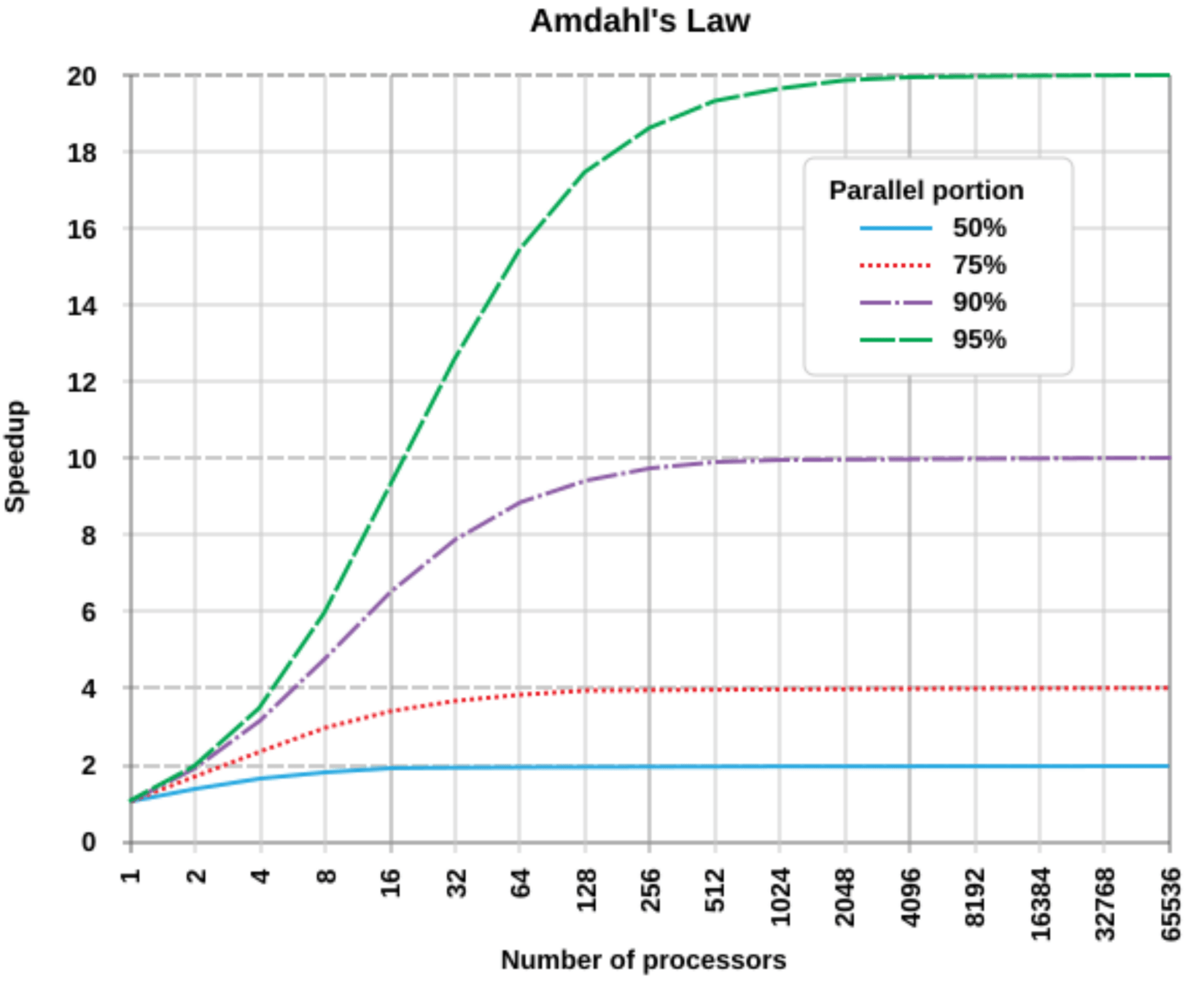
Amdahl's Law
-
Your ability to parallelize a program is limited by the serial parts:
-
\(S\) is the speedup
-
\(p\) is the parallel portion of the program
-
\(n\) is the number of processors
-
-
What is your expected speedup with 64 processors if 99.9% of your program can be parallelized?
David Mayerich
STIM Laboratory, University of Houston
S = \frac{1}{
(1-p)+\frac{p}{n}
}
S = \frac{1}{
(0.001)+\frac{0.999}{64}
}
\approx
60X
Gustafson's Law
-
Alternative approach gives more optimistic results:
\(S=1-p+pn\)-
\(S\) is the speedup
-
\(p\) is the parallel portion of the code
-
\(n\) is the number of processors
-
-
What is your expected speedup with 64 processors if 99.9% of your program can be parallelized?
\(0.001 + 0.999 \times 64 \approx 64X\)
David Mayerich
STIM Laboratory, University of Houston
-
Why different answers (60X vs. 64X)?
-
Ahmdal's law represents a fixed problem size
-
Gustafson's law assumes the parallel part will grow to fully occupy the available processors
How would this apply to our heat equation example?
D.2 Heat Equation
By STIM Laboratory