Efficient Global Planning for
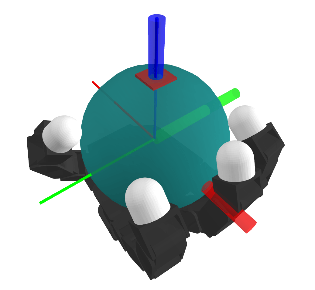
Contact-Rich Manipulation
Hyung Ju Terry Suh, MIT
Talk @KAIST
2024-02-08
Chapter 1. Introduction
What is manipulation?
Rigid-body manipulation: Move object from pose A to pose B
A
B
What is manipulation?
How hard could this be? Just pick and place!
Rigid-body manipulation: Move object from pose A to pose B
A
B
Beyond pick & place
[DRPTSE 2016]
[ZH 2022]
[SKPMAT 2022]
[JTCCG 2014]
[PSYT 2022]
[ST 2020]

How have we been making progress?
Some amazing progress made with RL / IL.
Reinforcement Learning
Imitation Learning
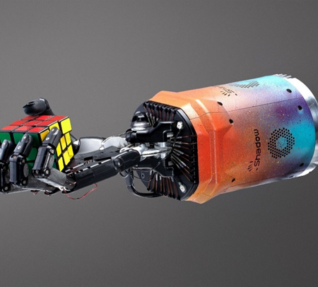
[OpenAI 2018]
[CFDXCBS 2023]
How have we been making progress?
Some amazing progress made with RL / IL.
Reinforcement Learning
Imitation Learning
[OpenAI 2018]
[CFDXCBS 2023]
But how do we generalize and scale to the complexity of manipulation?
Generalization vs. Specialization
Specialization
Generalization
RL / IL are specialists!
- Extremely good at solving one task
- Long turnaround time for new skill acquisition
Fixed object + Few Goals
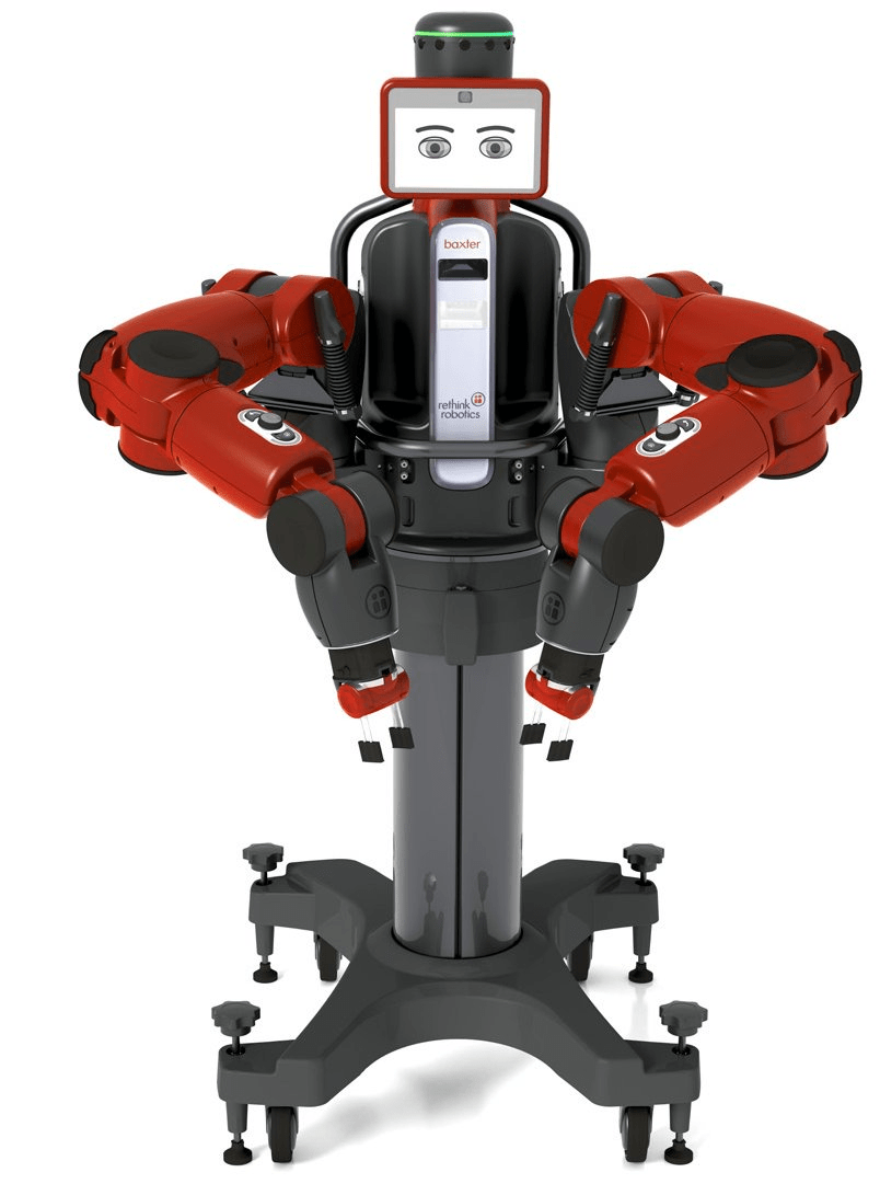
- What if we want different goals?
- What if the object shape changes?
- What if I have a different hand?
- What if I have a different environment?
How do we generalize?
Collect more data?
Secret Ingredient 1. Newton's Laws for Manipulation
Models Generalize!


Secret Ingredient 1. Newton's Laws for Manipulation
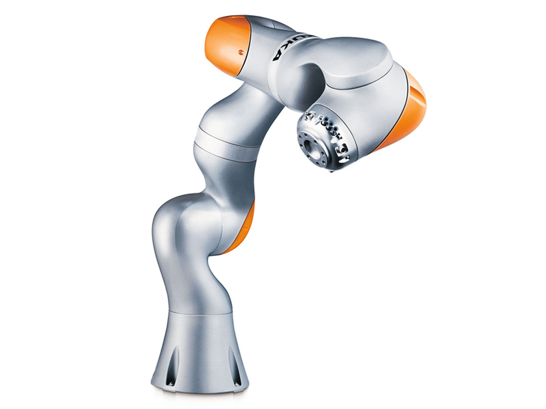
An Example of Generalization in Manipulation
How can we build "Newton's Laws" for contact-rich manipulation?
Models Generalize!
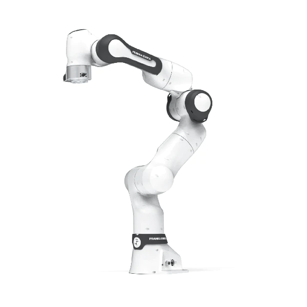
Differential Inverse Kinematics:
As long as you have the manipulator Jacobian, same control strategy works for every arm.
Secret Ingredient 2. Efficient Search for Manipulation
Specialization
Generalization
RL / IL are specialists!
- Extremely good at solving one task
- Long turnaround time for new skill acquisition
Fixed object + Few Goals
- What if we want different goals?
- What if the object shape changes?
- What if I have a different hand?
- What if I have a different environment?
Search allows for
combinatorial generalization
Inference
Offline Computation
Search
Online Computation
Secret Ingredient 2. Efficient Search for Manipulation
Specialization
Generalization
RL / IL
Search
Not Mutually Exclusive!
They beautifully help each other.
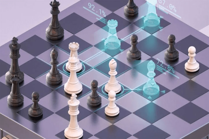
MuZero
[Deepmind 2019]
Search allows better exploration, data generation for inference.
Feedback Motion Planning
[Tedrake 2009]
Inference allows for hierarchies that can narrow down the search space
Inference
Offline Computation
Search
Online Computation
Story of how we've built this capability
What about different goals, shapes,
environments, and tasks?
Newton's Laws for Manipulation
Efficient Search

How do we generalize?
Status Quo
Keep collecting data.
We're willing to spend huge offline time,
but your inference time (online) will be short.
Give me a few amount of online time (on an order of a minute), I'll give you the answer.
Our Proposal.
Overview of the Talk
Chapter 1. Introduction
Chapter 2. What's hard about contact?
Chapter 3. Why is RL so good?
Chapter 4. Bringing lessons from RL
Chapter 5. Efficient Global Planning
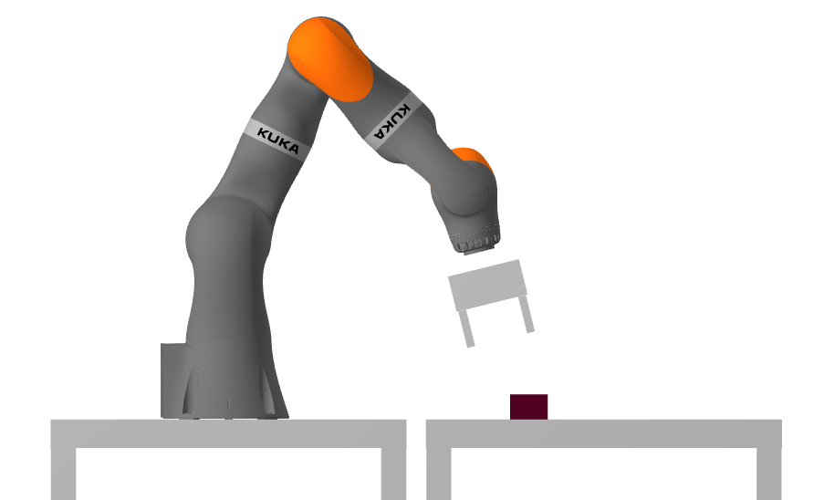
Chapter 2. What makes contact hard?
Planning through Contact: Problem Statement
System configuration as q
- Actuated degrees-of-freedom (Robot)
q^\mathrm{a}
Planning through Contact: Problem Statement
System configuration as q
- Actuated degrees-of-freedom (Robot)
- Unactuated degrees-of-freedom (Object)
q^\mathrm{u}
q^\mathrm{a}
Planning through Contact: Problem Statement
System configuration as
- Actuated degrees-of-freedom (Robot)
- Unactuated degrees-of-freedom (Object)
q^\mathrm{u}
q^\mathrm{a}
Robot commands as

q
u
Planning through Contact: Problem Statement
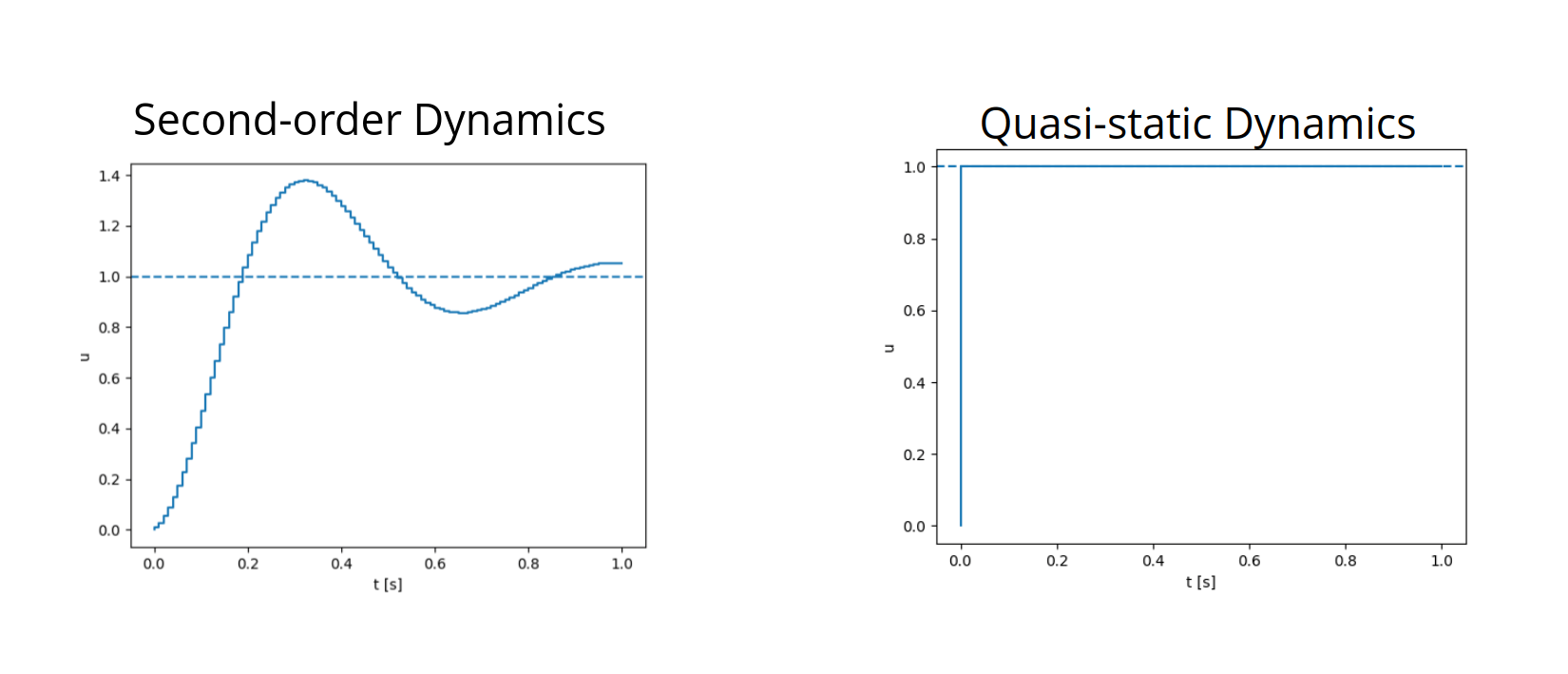
System Dynamics
q_+ = f(q,u)

f
We will assume quasistatic dynamics - velocities are very small in magnitude.
Planning through Contact: Problem Statement
\begin{aligned}
\text{find} \quad & u_0,u_1,\cdots,u_T, q_0,q_1,\cdots,q_{T+1} \\
\text{s.t.} \quad & q_0 = q_{initial} \\
& q^\mathrm{u}_T = q^\mathrm{u}_{goal} \\
& q_{t+1} = f(q_t, u_t)\quad \quad \forall t\in\{0,\cdots,T\}
\end{aligned}
Find a sequence of actions and configurations to drive object to goal configuration.
q_0
q_1
q_2
q_3
q_4
u_0
u_1
u_2
u_3
Solution Desiderata
Efficient Global Planning for
Highly Contact-Rich Systems
Fast Solution Time
Beyond Local Solutions
Contact Scalability
Why is this problem difficult?
\begin{aligned}
\mathrm{find} \quad & u_0, q_1\\
\text{s.t.} \quad & q_0 = q_{initial} \\
& q^\mathrm{u}_1 = q^\mathrm{u}_{goal} \\
& q_1 = f(q_0, u_0)
\end{aligned}
To get some intuition, let's simplify the problem a bit!
\begin{aligned}
\text{find} \quad & u_0,u_1,\cdots,u_T, q_0,q_1,\cdots,q_{T+1} \\
\text{s.t.} \quad & q_0 = q_{initial} \\
& q^\mathrm{u}_T = q^\mathrm{u}_{goal} \\
& q_{t+1} = f(q_t, u_t)\quad \quad \forall t\in\{0,\cdots,T\}
\end{aligned}
Original Problem
Horizon 1
Simplifying the Problem
To get some intuition, let's simplify the problem a bit!
\begin{aligned}
\mathrm{find} \quad & u_0, q_1\\
\text{s.t.} \quad & q_0 = q_{initial} \\
& q^\mathrm{u}_1 = q^\mathrm{u}_{goal} \\
& q_1 = f(q_0, u_0)
\end{aligned}
Horizon 1
Penalty on Terminal Constraint
\begin{aligned}
\text{find} \quad & u_0,u_1,\cdots,u_T, q_0,q_1,\cdots,q_{T+1} \\
\text{s.t.} \quad & q_0 = q_{initial} \\
& q^\mathrm{u}_T = q^\mathrm{u}_{goal} \\
& q_{t+1} = f(q_t, u_t)\quad \quad \forall t\in\{0,\cdots,T\}
\end{aligned}
Original Problem
\begin{aligned}
\min_{u_0,q_1} \quad & \|q_1^\mathrm{u} - q^\mathrm{u}_{goal}\|^2\\
\text{s.t.} \quad & q_0 = q_{initial} \\
& q_1^\mathrm{u} = f^\mathrm{u}(q_0, u_0)
\end{aligned}
Simplifying the Problem
\begin{aligned}
\text{find} \quad & u_0,u_1,\cdots,u_T, q_0,q_1,\cdots,q_{T+1} \\
\text{s.t.} \quad & q_0 = q_{initial} \\
& q^\mathrm{u}_T = q^\mathrm{u}_{goal} \\
& q_{t+1} = f(q_t, u_t)\quad \quad \forall t\in\{0,\cdots,T\}
\end{aligned}
Original Problem
Simplified Problem
\begin{aligned}
\mathrm{find} \quad & u_0, q_1\\
\text{s.t.} \quad & q_0 = q_{initial} \\
& q^\mathrm{u}_1 = q^\mathrm{u}_{goal} \\
& q_1 = f(q_0, u_0)
\end{aligned}
Horizon 1
\begin{aligned}
\min_{u_0} \quad & \|f^\mathrm{u}(q_0,u_0) - q^\mathrm{u}_{goal}\|^2
\end{aligned}
\begin{aligned}
\min_{u_0,q_1} \quad & \|q_1^\mathrm{u} - q^\mathrm{u}_{goal}\|^2\\
\text{s.t.} \quad & q_0 = q_{initial} \\
& q_1^\mathrm{u} = f^\mathrm{u}(q_0, u_0)
\end{aligned}
Penalty on Terminal Constraint
Equivalent to
Toy Problem
Simplified Problem
\begin{aligned}
\min_{u_0} \quad & \|f^\mathrm{u}(q_0,u_0) - q^\mathrm{u}_{goal}\|^2
\end{aligned}
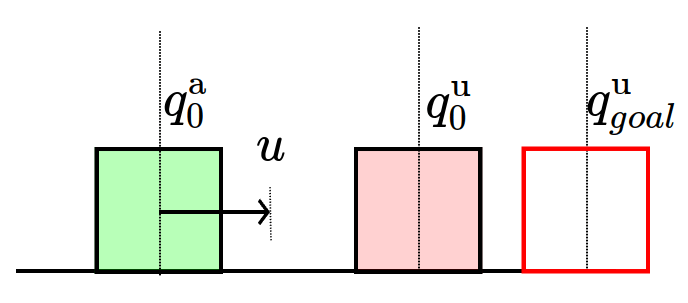
Given some initial and goal configuration, which action minimizes distance to the goal configuration?
\begin{aligned}
q_0
\end{aligned}
\begin{aligned}
q^\mathrm{u}_{goal}
\end{aligned}
\begin{aligned}
q^\mathrm{u}_0
\end{aligned}
\begin{aligned}
q^\mathrm{a}_0
\end{aligned}
\begin{aligned}
q^\mathrm{u}_{goal}
\end{aligned}
\begin{aligned}
u
\end{aligned}
Toy Problem
Simplified Problem
\begin{aligned}
\min_{u_0} \quad & \frac{1}{2}\|f^\mathrm{u}(q_0,u_0) - q^\mathrm{u}_{goal}\|^2
\end{aligned}
\begin{aligned}
q^\mathrm{u}_0
\end{aligned}
\begin{aligned}
q^\mathrm{a}_0
\end{aligned}
\begin{aligned}
q^\mathrm{u}_{goal}
\end{aligned}
\begin{aligned}
u
\end{aligned}
Consider simple gradient descent,
\begin{aligned}
u \leftarrow u - \eta \nabla_u \textstyle\frac{1}{2} \|f^\mathrm{u}(q_0,u_0) - q^\mathrm{u}_{goal}\|^2
\end{aligned}
\begin{aligned}
u \leftarrow u - \eta \left[f^\mathrm{u}(q_0,u_0) - q^\mathrm{u}_{goal}\right]{\color{red} \nabla_u f^\mathrm{u}(q_0,u_0)}
\end{aligned}
Toy Problem
Simplified Problem
\begin{aligned}
\min_{u_0} \quad & \frac{1}{2}\|f^\mathrm{u}(q_0,u_0) - q^\mathrm{u}_{goal}\|^2
\end{aligned}
Consider simple gradient descent,
\begin{aligned}
u \leftarrow u - \eta \nabla_u \textstyle\frac{1}{2} \|f^\mathrm{u}(q_0,u_0) - q^\mathrm{u}_{goal}\|^2
\end{aligned}
\begin{aligned}
u \leftarrow u - \eta \left[f^\mathrm{u}(q_0,u_0) - q^\mathrm{u}_{goal}\right]{\color{red} \nabla_u f^\mathrm{u}(q_0,u_0)}
\end{aligned}
\begin{aligned}
q^\mathrm{u}_1=f^\mathrm{u}(q_0,u_0)
\end{aligned}
\begin{aligned}
u_0
\end{aligned}
Dynamics of the system
No Contact
Contact
\begin{aligned}
q^\mathrm{u}_0
\end{aligned}
\begin{aligned}
q^\mathrm{a}_0
\end{aligned}
\begin{aligned}
q^\mathrm{u}_{goal}
\end{aligned}
\begin{aligned}
u
\end{aligned}
Toy Problem
Simplified Problem
\begin{aligned}
\min_{u_0} \quad & \frac{1}{2}\|f^\mathrm{u}(q_0,u_0) - q^\mathrm{u}_{goal}\|^2
\end{aligned}
Consider simple gradient descent,
\begin{aligned}
u \leftarrow u - \eta \nabla_u \textstyle\frac{1}{2} \|f^\mathrm{u}(q_0,u_0) - q^\mathrm{u}_{goal}\|^2
\end{aligned}
\begin{aligned}
u \leftarrow u - \eta \left[f^\mathrm{u}(q_0,u_0) - q^\mathrm{u}_{goal}\right]{\color{red} \nabla_u f^\mathrm{u}(q_0,u_0)}
\end{aligned}
\begin{aligned}
q^\mathrm{u}_1=f^\mathrm{u}(q_0,u_0)
\end{aligned}
\begin{aligned}
u_0
\end{aligned}
Dynamics of the system
No Contact
Contact
The gradient is zero if there is no contact!
The gradient is zero if there is no contact!
\begin{aligned}
q^\mathrm{u}_0
\end{aligned}
\begin{aligned}
q^\mathrm{a}_0
\end{aligned}
\begin{aligned}
q^\mathrm{u}_{goal}
\end{aligned}
\begin{aligned}
u
\end{aligned}
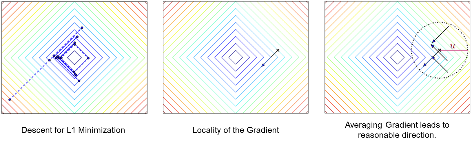
Local gradient-based methods easily get stuck due to the flat / non-smooth nature of the landscape
Previous Approaches to Tackling the Problem
Why don't we search more globally for a locally optimal action subject to each contact mode?
In no-contact, run gradient descent.
In contact, run gradient descent.
Contact
No Contact
\begin{aligned}
u_0
\end{aligned}
Cost
Previous Approaches to Tackling the Problem
Why don't we search more globally for a locally optimal action subject to each contact mode?
In no-contact, run gradient descent.
In contact, run gradient descent.
Mixed Integer Programming
Mode Enumeration
Active Set Approach

[MDGBT 2017]
[HR 2016]
[CHHM 2022]
[AP 2022]
Contact
No Contact
\begin{aligned}
u_0
\end{aligned}
Cost
Problems with Mode Enumeration
System
Number of Modes
\begin{aligned}
N = 2
\end{aligned}
\begin{aligned}
N = 3^{\binom{9}{2}}
\end{aligned}
No Contact
Sticking Contact
Sliding Contact
Number of potential active contacts
Problems with Mode Enumeration
System
Number of Modes
\begin{aligned}
N = 3^{\binom{20}{2}} \approx 4.5 \times 10^{90}
\end{aligned}
The number of modes scales terribly with system complexity
\begin{aligned}
N = 2
\end{aligned}
\begin{aligned}
N = 3^{\binom{9}{2}}
\end{aligned}
No Contact
Sticking Contact
Sliding Contact
Number of potential active contacts
Mixed Integer Approaches


Efficient Global Planning for
Highly Contact-Rich Systems
Fast Solution Time
Beyond Local Solutions
Contact Scalability
Chapter 3. What makes RL so good?
Reinforcement Learning
Efficient Global Planning for
Highly Contact-Rich Systems
Fast Solution Time
Beyond Local Solutions
Contact Scalability
Why is RL so good?
Why are model-based planning methods doing not as well?
How does RL power through these problems?
Reinforcement Learning fundamentally considers a stochastic objective
\begin{aligned}
\min_{u_0} \quad & \frac{1}{2}\|f^\mathrm{u}(q_0,u_0) - q^\mathrm{u}_{goal}\|^2
\end{aligned}
Previous Formulations
\begin{aligned}
\min_{u_0} \quad & \frac{1}{2}{\color{red} \mathbb{E}_{w\sim \rho}}\|f^\mathrm{u}(q_0,u_0 {\color{red} + w}) - q^\mathrm{u}_{goal}\|^2
\end{aligned}
Reinforcement Learning
Contact
No Contact
Cost
\begin{aligned}
u_0
\end{aligned}
How does RL power through these problems?
\begin{aligned}
\min_{u_0} \quad & \frac{1}{2}\|f^\mathrm{u}(q_0,u_0) - q^\mathrm{u}_{goal}\|^2
\end{aligned}
Previous Formulations
Reinforcement Learning
Contact
No Contact
Cost
\begin{aligned}
u_0
\end{aligned}
\begin{aligned}
& \min_{u_0}\quad \frac{1}{2}{\color{red} \mathbb{E}_{w\sim \rho}}\|f^\mathrm{u}(q_0,u_0 {\color{red} + w}) - q^\mathrm{u}_{goal}\|^2 \\
=& \min_{u_0}\quad \frac{1}{2} \mathbb{E}_{w\sim\rho}\left[{\color{blue} F}(u_0 + w)\right]
\end{aligned}
Contact
No Contact
Averaged
\begin{aligned}
u_0
\end{aligned}
Randomized smoothing
regularizes landscapes
Cost
How does RL power through these problems?
\begin{aligned}
\min_{u_0} \quad & \frac{1}{2}\|f^\mathrm{u}(q_0,u_0) - q^\mathrm{u}_{goal}\|^2
\end{aligned}
Previous Formulations
Reinforcement Learning
\begin{aligned}
& \min_{u_0}\quad \frac{1}{2}{\color{red} \mathbb{E}_{w\sim \rho}}\|f^\mathrm{u}(q_0,u_0 {\color{red} + w}) - q^\mathrm{u}_{goal}\|^2 \\
=& \min_{u_0}\quad \frac{1}{2} \mathbb{E}_{w\sim\rho}\left[{\color{blue} F}(u_0 + w)\right]
\end{aligned}
Contact
No Contact
Averaged
\begin{aligned}
u_0
\end{aligned}
Cost
\begin{aligned}
q^\mathrm{u}_0
\end{aligned}
\begin{aligned}
q^\mathrm{a}_0
\end{aligned}
\begin{aligned}
q^\mathrm{u}_{goal}
\end{aligned}
\begin{aligned}
u
\end{aligned}
Some samples end up in contact, some samples do not!
No consideration of modes.
Randomized smoothing
regularizes landscapes
Original Problem
\begin{aligned}
\min_\theta V(\theta)
\end{aligned}
Long-horizon problems involving contact can have terrible landscapes.
How does RL power through these problems?
[SSZT 2022]
Smoothing of Value Functions.
Smooth Surrogate
\begin{aligned}
\min_\theta \mathbb{E}_w V(\theta + w)
\end{aligned}
The benefits of smoothing are much more pronounced in the value smoothing case.
Beautiful story - noise sometimes regularizes the problem, developing into helpful bias.
[SSZT 2022]
Computation of Gradients
But how do we take gradients through a stochastic objective?
First-Order Gradient Estimator
\begin{aligned}
\nabla_\theta \mathbb{E}_w V(\theta + w) & = \mathbb{E}_w \nabla_\theta V(\theta + w) \\
& = \frac{1}{N}\sum^N_{i=1}\nabla_\theta V(\theta + w_i)
\end{aligned}
Zeroth-Order Gradient Estimator
\begin{aligned}
\nabla_\theta \mathbb{E}_w V(\theta + w) & = \frac{1}{\sigma^2}\mathbb{E}_w [V(\theta + w)w] \\
& = \frac{1}{N}\sum^N_{i=1}\frac{1}{\sigma^2} V(\theta + w_i)w_i
\end{aligned}
\begin{aligned}
\nabla_\theta \mathbb{E}_w V(\theta + w)
\end{aligned}
Reparametrization Gradient
Gradient Sampling
REINFORCE
Score Function Gradient
Likelihood Ratio Gradient
Stein Gradient Estimator
Common Lesson in Stochastic Optimization
Analytic Expression
First-Order Gradient Estimator
Zeroth-Order Gradient Estimator
- Requires differentiability over dynamics, reward, policy.
- Generally lower variance.
- Only requires zeroth-order oracle (value of f)
- High variance.
Structure Requirements
Performance / Efficiency
Possible for only few cases
First-Order Policy Search with Differentiable Simulation
Policy Gradient Methods in RL (REINFORCE / TRPO / PPO)
- Requires differentiability over dynamics, reward, policy.
- Generally lower variance.
- Only requires zeroth-order oracle (value of f)
- High variance.
Structure Requirements
Performance / Efficiency
Turns out there is an important question hidden here regarding the utility of differentiable simulators.
Common Lesson in Stochastic Optimization
Do Differentiable Simulators Give Better Policy Gradients?
Very important question for RL, as it promises lower variance, faster convergence rates, and more sample efficiency.
What do we mean by better?
Bias
Variance
Common lesson from stochastic optimization:
1. Both are unbiased under sufficient regularity conditions
2. First-order generally has less variance than zeroth order.
We show two cases where the commonly accepted wisdom is not true.
Pathologies of Differentiable RL
Bias
Variance
Common lesson from stochastic optimization:
1. Both are unbiased under sufficient regularity conditions
2. First-order generally has less variance than zeroth order.
Bias
Variance
Bias
Variance
We show two cases where the commonly accepted wisdom is not true.
1st Pathology: First-Order Estimators CAN be biased.
2nd Pathology: First-Order Estimators can have MORE
variance than zeroth-order.
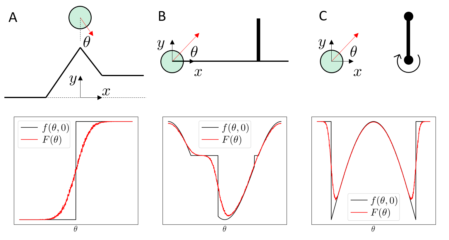
Bias from Discontinuities
1st Pathology: First-Order Estimators CAN be biased.
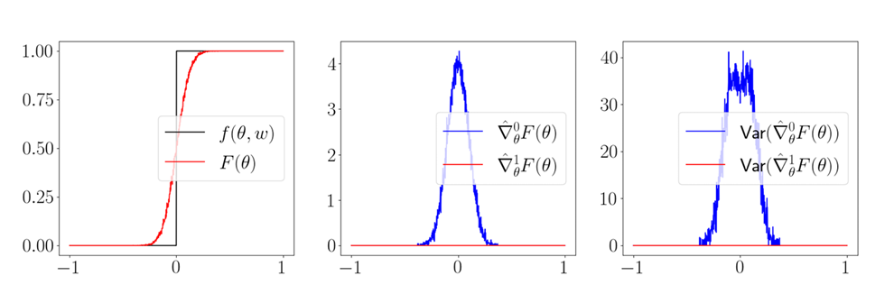
\begin{aligned}
\nabla_\theta \mathbb{E}_w f(\theta + w) & = \mathbb{E}_w f(\theta + w) = \frac{1}{N}\sum^N_{i=1}\nabla_\theta f(\theta + w_i)
\end{aligned}
Note that empirical variance is also zero for first-order!
Empirical Bias
Happens for near-discontinuities as well!
\begin{aligned}
\textbf{Var}_\theta\left[{\color{blue}\frac{1}{N}\frac{1}{\sigma^2}\sum^N_{i=1}V(\theta + w_i)w_i}\right] \leq \frac{\dim \theta}{N\sigma^2}\max_w\|V(\theta + w)\|^2_2
\end{aligned}
\begin{aligned}
\textbf{Var}_\theta\left[{\color{red}\frac{1}{N}\sum^N_{i=1}\nabla_\theta V(\theta + w_i)}\right] \leq \frac{1}{N}\max_w \|\nabla_\theta V(\theta + w)\|^2_2
\end{aligned}
Scales with Gradient
Scales with Function Value
Scales with dimension of decision variables.
Variance of First-Order Estimators
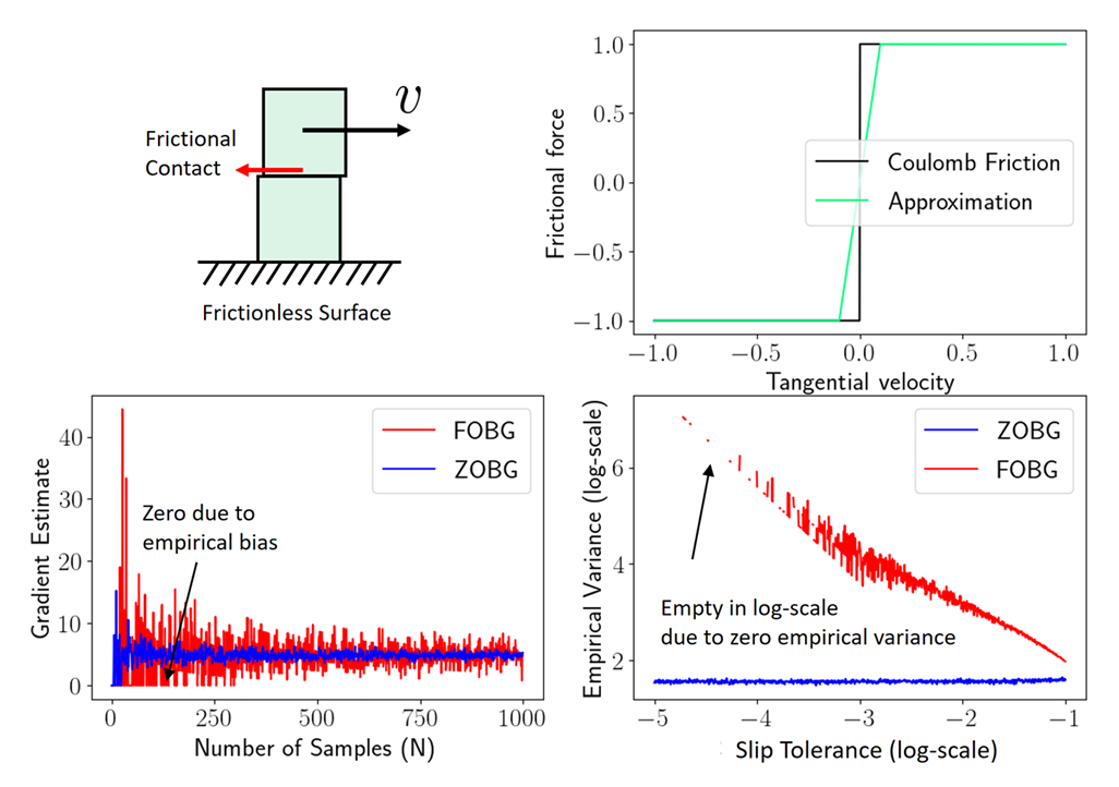
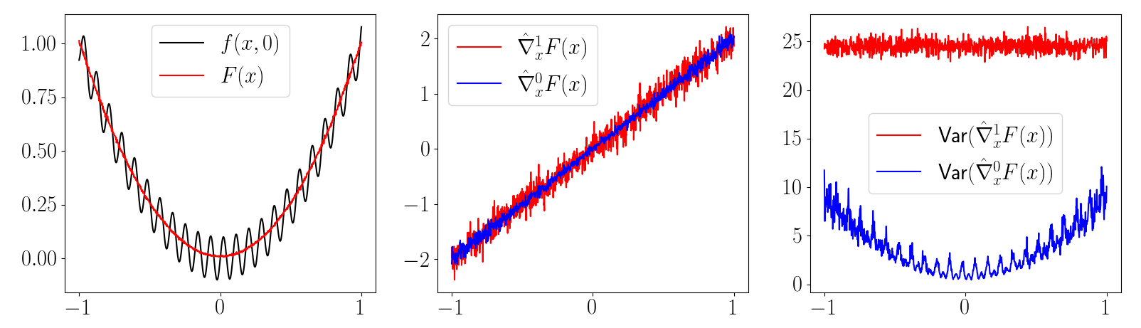
2nd Pathology: First-order Estimators CAN have more variance than zeroth-order ones.
High-Variance Events
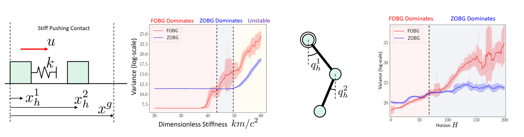
Case 1. Persistent Stiffness
Case 2. Chaos
Few Important Lessons
Why does RL do better on these problems?
Randomized Smoothing: Regularization effects of stochasticity
Zeroth-Order Gradients are surprisingly robust
- Chaining first-order gradients explode / vanish.
- First order gradients suffer from empirical bias under stiff dynamics.
Chapter 4. Bringing lessons from RL
Few Important Lessons
How do we do better?
Regularizing Effects of Stochasticity
Contact problems require some smoothing regularization
Stiff dynamics causes empirical bias / gradient explosion.
Are we writing down our models in the right way?
Chaining first-order gradients explode / vanish
Let's avoid single shooting.
Newton's Laws for Manipulation
Are we writing down the models in the right way?
Newton's Laws for Manipulation

Are we writing down the models in the right way?
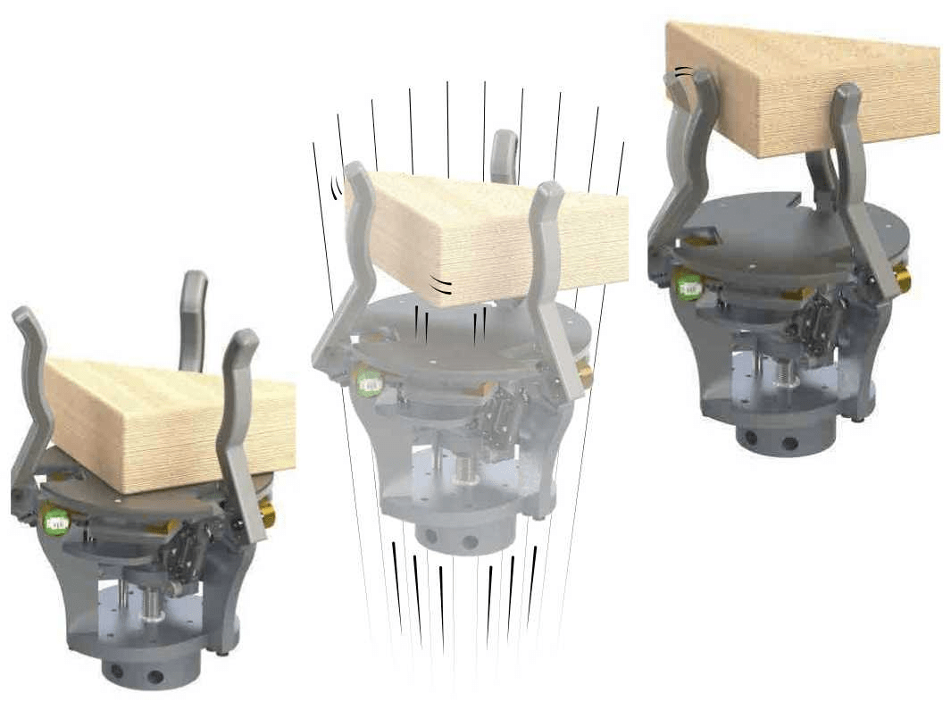
How did we predict this?
Results vary, but we always know what's NOT going to happen.
Newton's Laws for Manipulation
\begin{aligned}
q^\mathrm{a}_1
\end{aligned}
\begin{aligned}
q^\mathrm{a}_0 + u
\end{aligned}
No Contact
Contact
Newton's laws for manipulation seem much more like constrained optimization problems!
\begin{aligned}
q^\mathrm{a}_0
\end{aligned}
\begin{aligned}
u
\end{aligned}
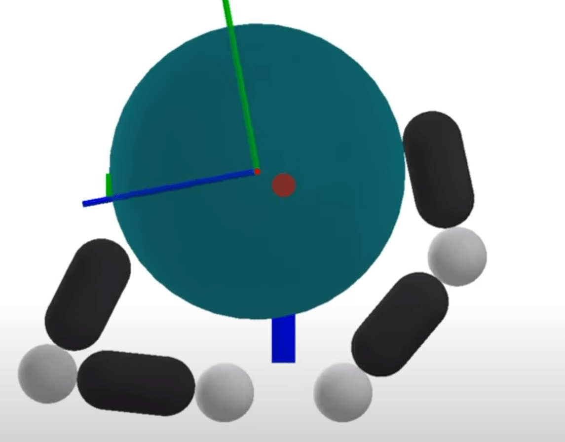
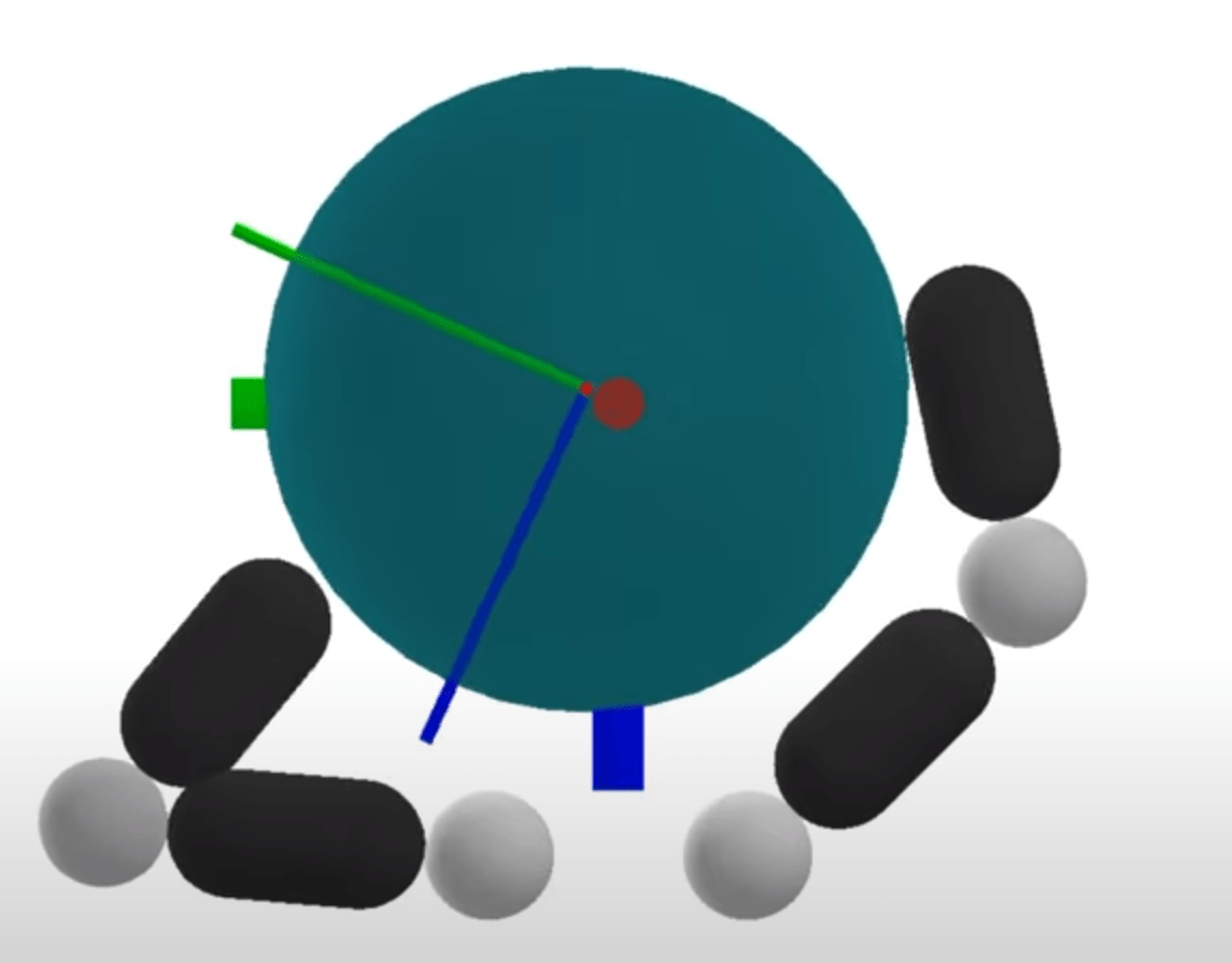
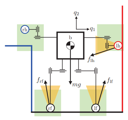
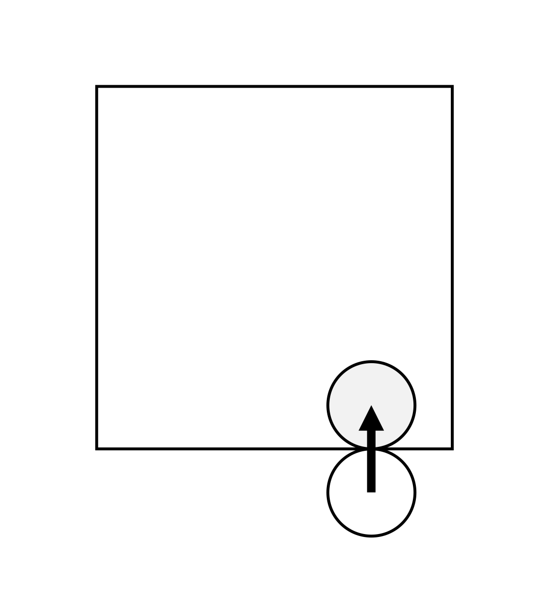
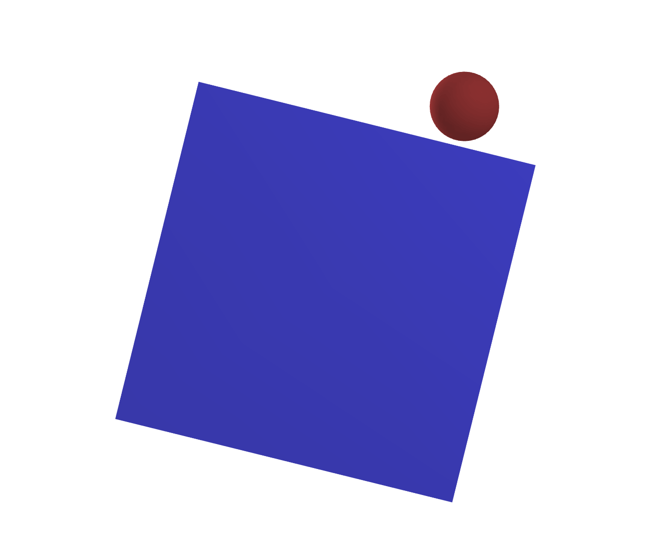
Example: Box vs. wall
Commanded next position
Actual next position
Cannot penetrate into the wall
Constrained-based Simulation
\begin{aligned}
\min_{{\color{blue} q^\mathrm{a}_1}}& \quad \frac{1}{2}k\|{\color{red} q^\mathrm{a}_0 + u_0} - {\color{blue} q^\mathrm{a}_1}\|^2 \\
\text{s.t.} &\quad {\color{blue} q^\mathrm{a}_1} \geq 0
\end{aligned}
\begin{aligned}
k
\end{aligned}
Interpretation with KKT Conditions
KKT Conditions
\begin{aligned}
k(q^\mathrm{a}_0 + u - q^\mathrm{a}_1) & = \lambda\\
q^\mathrm{a}_1 & \geq 0 \\
\lambda & \geq 0 \\
q^\mathrm{a}_1 \lambda & = 0
\end{aligned}
(Stationarity)
(Primal Feasibility)
(Dual Feasibility)
(Complementary Slackness)
Example: Box vs. wall
Commanded next position
Actual next position
Cannot penetrate into the wall
Constrained-based Simulation
\begin{aligned}
\min_{{\color{blue} q^\mathrm{a}_1}}& \quad \frac{1}{2}k\|{\color{red} q^\mathrm{a}_0 + u_0} - {\color{blue} q^\mathrm{a}_1}\|^2 \\
\text{s.t.} &\quad {\color{blue} q^\mathrm{a}_1} \geq 0
\end{aligned}
Contact Constraints naturally encoded as
optimality conditions
\begin{aligned}
q^\mathrm{a}_0
\end{aligned}
\begin{aligned}
u
\end{aligned}
\begin{aligned}
k
\end{aligned}
\begin{aligned}
\lambda
\end{aligned}
Newton's Laws for Manipulation
\begin{aligned}
\min_{{\color{blue} q^\mathrm{a}_1}}& \quad \frac{1}{2}k\|{\color{red} q^\mathrm{a}_0 + u_0} - {\color{blue} q^\mathrm{a}_1}\|^2 \\
\text{s.t.} &\quad {\color{blue} q^\mathrm{a}_1} \geq 0
\end{aligned}
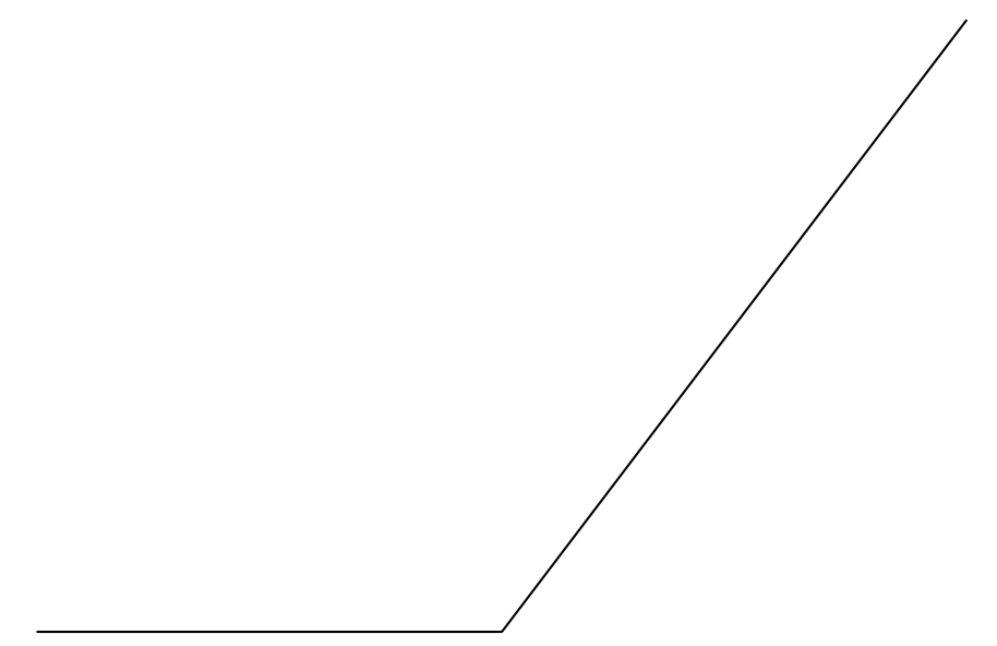
Penalty Method
Optimization-based Dynamics
- Prone to stiff dynamics
- Oscillations can cause inefficiencies for chaining gradients
- Less stiff dynamics
- Long-horizon gradients by jumping through equilibrium
How you simulate matters for gradients!
Newton's Laws for Manipulation
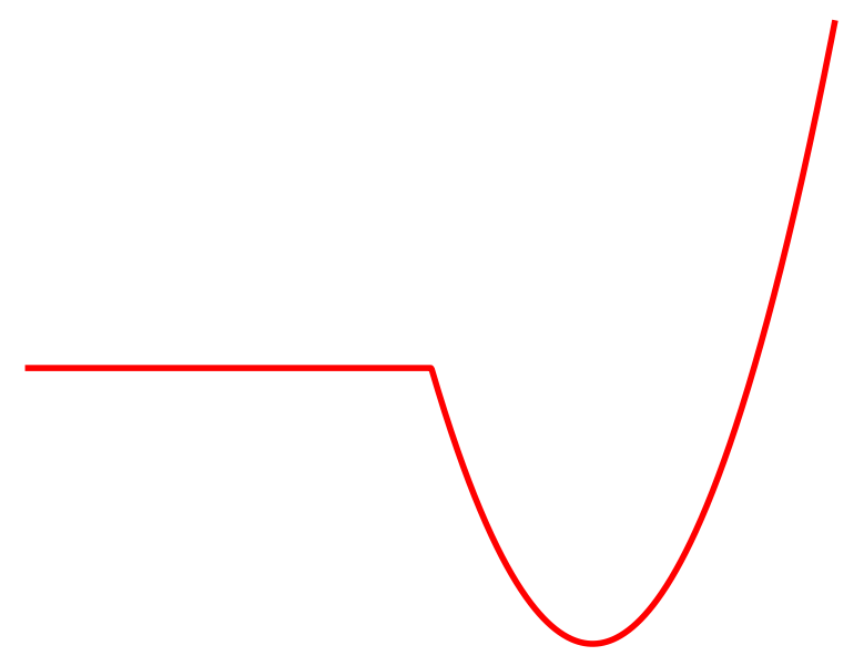
Log-Barrier Relaxation
\begin{aligned}
\min_{{\color{blue} q^\mathrm{a}_1}}& \quad \frac{1}{2}\|{\color{red} q^\mathrm{a}_0 + u_0} - {\color{blue} q^\mathrm{a}_1}\|^2 - \kappa^{-1}\log {\color{blue} q^\mathrm{a}_1}
\end{aligned}
\begin{aligned}
\min_{{\color{blue} q^\mathrm{a}_1}}& \quad \frac{1}{2}k\|{\color{red} q^\mathrm{a}_0 + u_0} - {\color{blue} q^\mathrm{a}_1}\|^2 \\
\text{s.t.} &\quad {\color{blue} q^\mathrm{a}_1} \geq 0
\end{aligned}
Optimization-based Dynamics
Randomized smoothing
Barrier smoothing
\begin{aligned}
q^\mathrm{a}_0 + u
\end{aligned}
\begin{aligned}
q^\mathrm{a}_1
\end{aligned}
Optimization-based dynamics can be regularized easily!
(without Monte Carlo)
Differentiating with Sensitivity Analysis
How do we obtain the gradients from an optimization problem?
\begin{aligned}
\frac{\partial q^{\star\mathrm{a}}_1}{\partial u_0}
\end{aligned}
\begin{aligned}
\min_{{\color{blue} q^\mathrm{a}_1}}& \quad \frac{1}{2}\|{\color{red} q^\mathrm{a}_0 + u_0} - {\color{blue} q^\mathrm{a}_1}\|^2 - \kappa^{-1}\log {\color{blue} q^\mathrm{a}_1}
\end{aligned}

Differentiating with Sensitivity Analysis
How do we obtain the gradients from an optimization problem?
\begin{aligned}
\frac{\partial q^{\mathrm{a}\star}_1}{\partial u_0}
\end{aligned}
\begin{aligned}
q^\mathrm{a}_0 + u - q^{\mathrm{a}\star}_1 - \kappa^{-1}\frac{1}{q^{\mathrm{a}\star}_1} = 0
\end{aligned}
Differentiate through the optimality conditions!
Stationarity Condition
Implicit Function Theorem
\begin{aligned}
\left[1 + \kappa^{-1}\frac{1}{(q^{\mathrm{a}\star}_1)^2}\right]\frac{\partial q^{\mathrm{a}\star}}{\partial u_0} = 1
\end{aligned}
Differentiate by u
\begin{aligned}
\min_{{\color{blue} q^\mathrm{a}_1}}& \quad \frac{1}{2}\|{\color{red} q^\mathrm{a}_0 + u_0} - {\color{blue} q^\mathrm{a}_1}\|^2 - \kappa^{-1}\log {\color{blue} q^\mathrm{a}_1}
\end{aligned}
Differentiating with Sensitivity Analysis
[HLKM 2023]
[MBMSHNCRVM 2020]
[PSYT 2023]
How do we obtain the gradients from an optimization problem?
\begin{aligned}
\frac{\partial q^{\mathrm{a}\star}_1}{\partial u_0}
\end{aligned}
\begin{aligned}
q^\mathrm{a}_0 + u - q^{\mathrm{a}\star}_1 - \kappa^{-1}\frac{1}{q^{\mathrm{a}\star}_1} = 0
\end{aligned}
Differentiate through the optimality conditions!
Stationarity Condition
Implicit Function Theorem
\begin{aligned}
\left[1 + \kappa^{-1}\frac{1}{(q^{\mathrm{a}\star}_1)^2}\right]\frac{\partial q^{\mathrm{a}\star}_1}{\partial u_0} = 1
\end{aligned}
Differentiate by u
\begin{aligned}
\min_{{\color{blue} q^\mathrm{a}_1}}& \quad \frac{1}{2}\|{\color{red} q^\mathrm{a}_0 + u_0} - {\color{blue} q^\mathrm{a}_1}\|^2 - \kappa^{-1}\log {\color{blue} q^\mathrm{a}_1}
\end{aligned}
How have we learned from RL?
Lessons from RL
Model-based Remedy
-
Contact requires smoothing regularization
-
First-order gradients suffer from empirical bias under stiff dynamics
-
Chaining first-order gradients explode / vanish
\begin{aligned}
\min_{{\color{blue} q^\mathrm{a}_1}}& \quad \frac{1}{2}\|{\color{red} q^\mathrm{a}_0 + u_0} - {\color{blue} q^\mathrm{a}_1}\|^2 - \kappa^{-1}\log {\color{blue} q^\mathrm{a}_1}
\end{aligned}
-
Log-barrier relaxation provides smoothing regularization
-
Log-barrier smoothing requires no Monte Carlo estimation, and gradient is accurate.
-
Optimization-based dynamics provide longer-horizon gradients that leads to less explosion.
\begin{aligned}
\min_\theta \mathbb{E}_w V(\theta + w)
\end{aligned}
Gradient-based Optimization with Dynamics Smoothing
\begin{aligned}
\min_{u_{0:T}, q_{0:T}} \quad & \frac{1}{2}\|q_T^\mathrm{u} - q^\mathrm{u}_{goal}\|^2 \\
& q_{t+1} = \mathbb{E}_{w_t\sim\rho}\left[f(q_t, u_t)\right] \\
& q_0 = q_{initial}
\end{aligned}
\begin{aligned}
\min_{u_0} \quad & \frac{1}{2}\|f^\mathrm{u}(q_0,u_0) - q^\mathrm{u}_{goal}\|^2
\end{aligned}
Single Horizon
Single Horizon
Multi-Horizon
Scales extremely well in highly-rich contact
Efficient solutions in ~10s.
Efficient Global Planning for
Highly Contact-Rich Systems
Fast Solution Time
Beyond Local Solutions
Contact Scalability
[PCT 2014]
[MTP 2012]
[SPT 2022]
Gradient-based Optimization with Dynamics Smoothing
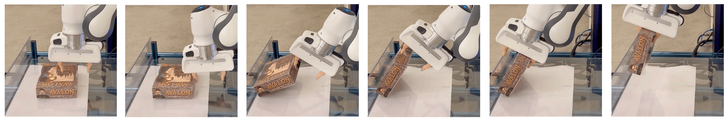
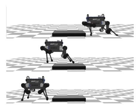
Fundamental Limitations with Local Search
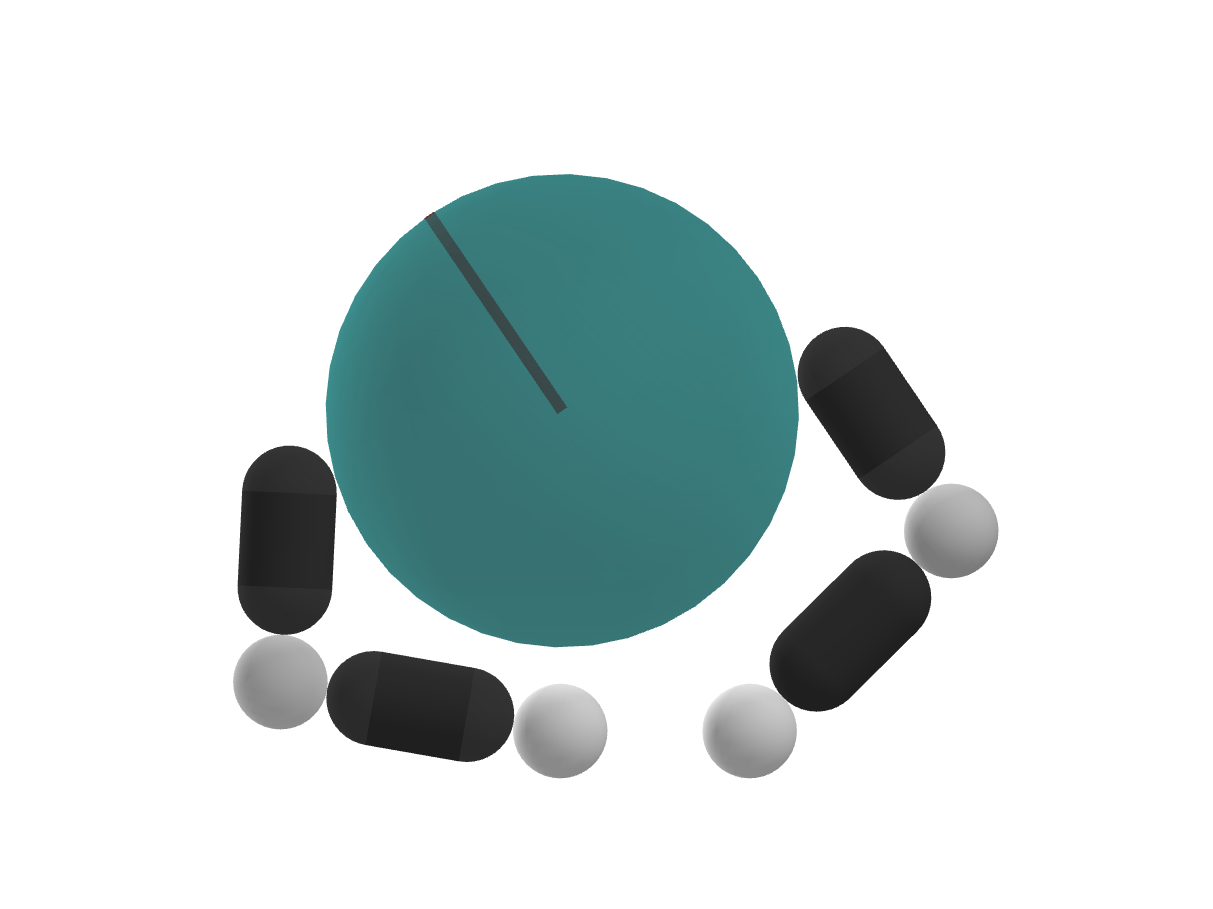
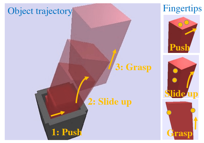
How do we push in this direction?
How do we rotate further in presence of joint limits?
Highly non-local movements are required to solve these problems
Chapter 5. Efficient Global Search
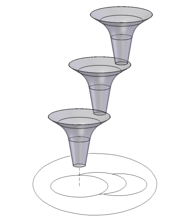
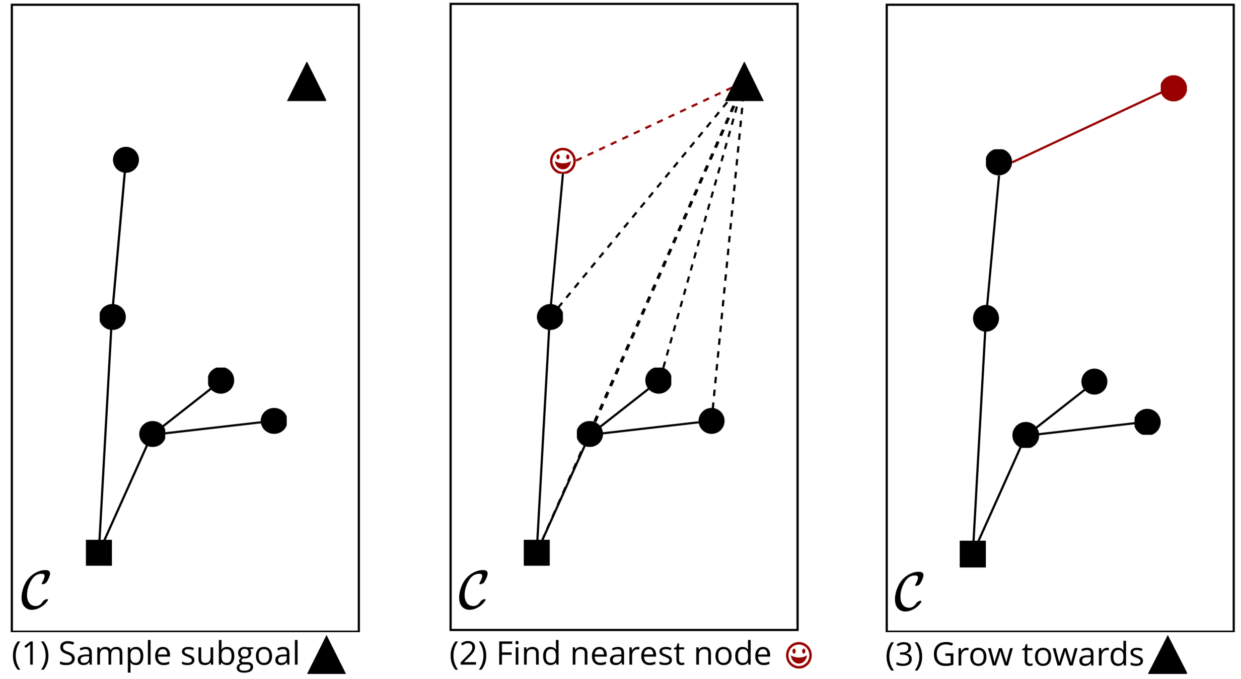
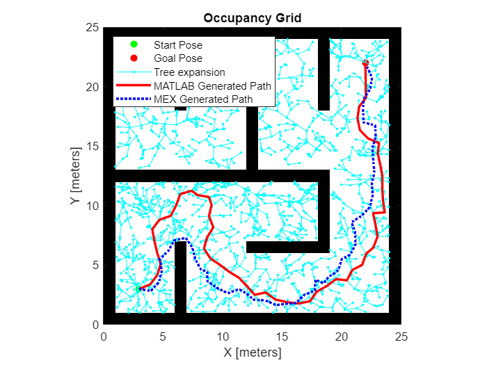
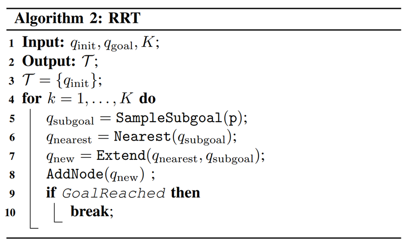
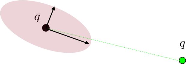
Rapidly Exploring Random Tree (RRT) Algorithm
Figure Adopted from Tao Pang's Thesis Defense, MIT, 2023
\mathcal{C}
(1) Sample subgoal
\mathcal{C}
(2) Find nearest node
\mathcal{C}
(3) Grow towards
Rapidly Exploring Random Tree (RRT) Algorithm
, "Planning Algorithms", Cambridge University Press , 2006.
RRT for Dynamics
Works well for Euclidean spaces. Why is it hard to use for dynamical systems?
RRT for Dynamics
Works well for Euclidean spaces. Why is it hard to use for dynamical systems?
What is "Nearest" in a dynamical system?
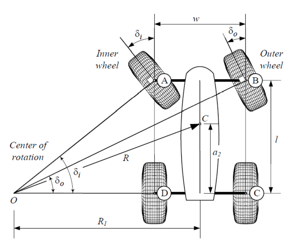
Closest in Euclidean space might not be closest for dynamics.
Rajamani et al., "Vehicle Dynamics"
SDW 2018
RRT for Dynamics
Works well for Euclidean spaces. Why is it hard to use for dynamical systems?
How do we "grow towards" a chosen subgoal?
Need to find actions (inputs) that would drive the system to the chosen subgoal.
Rajamani et al., "Vehicle Dynamics"
SDW 2018
RRT for Dynamics
Works well for Euclidean spaces. Why is it hard to use for dynamical systems?
How do we "grow towards" a chosen subgoal?
Note that these decisions are coupled
SDW 2018
Rajamani et al., "Vehicle Dynamics"
RRT for Dynamics
How do we "grow towards" a chosen subgoal?
\begin{aligned}
q^\mathrm{u}_0
\end{aligned}
\begin{aligned}
q^\mathrm{a}_0
\end{aligned}
\begin{aligned}
q^\mathrm{u}_{goal}
\end{aligned}
\begin{aligned}
u
\end{aligned}
\begin{aligned}
\min_{u_0} \quad & \frac{1}{2}\|f^\mathrm{u}(q_0,u_0) - q^\mathrm{u}_{goal}\|^2
\end{aligned}
We already know how to do this!
Inverse Dynamics
A Dynamically Consistent Distance Metric
What is the right distance metric
\begin{aligned}
d({\color{blue} q^\mathrm{u}_{goal}}; {\color{red} q_0})
\end{aligned}
\begin{aligned}
\color{blue} q^\mathrm{u}_{goal}
\end{aligned}
Fix some nominal values for ,
How far is from ?
\begin{aligned}
\color{red} q_0
\end{aligned}
\begin{aligned}
\color{red} q_0
\end{aligned}
A Dynamically Consistent Distance Metric
What is the right distance metric
The least amount of "Effort"
to reach the goal
\begin{aligned}
d({\color{blue} q^\mathrm{u}_{goal}}; {\color{red} q_0})
\end{aligned}
\begin{aligned}
\color{blue} q^\mathrm{u}_{goal}
\end{aligned}
Fix some nominal values for ,
How far is from ?
\begin{aligned}
\color{red} q_0
\end{aligned}
\begin{aligned}
\color{red} q_0
\end{aligned}
A Dynamically Consistent Distance Metric
\begin{aligned}
\color{blue} q^\mathrm{u}_{goal}
\end{aligned}
\begin{aligned}
d({\color{blue} q^\mathrm{u}_{goal}}; {\color{red} q_0})
\end{aligned}
What is the right distance metric
\begin{aligned}
\min_{u_0} \quad & \frac{1}{2}\|u_0\|^2 \\
\text{s.t.}\quad & f^\mathbf{u}({\color{red}q_0},u_0) = {\color{blue} q^\mathrm{u}_{goal}}
\end{aligned}
What is the right distance metric
\begin{aligned}
d({\color{blue} q^\mathrm{u}_{goal}}; {\color{red} q_0}) =
\end{aligned}
Fix some nominal values for ,
How far is from ?
\begin{aligned}
\color{red} q_0
\end{aligned}
\begin{aligned}
\color{red} q_0
\end{aligned}
The least amount of "Effort"
to reach the goal
\begin{aligned}
\color{red} q_0
\end{aligned}
A Dynamically Consistent Distance Metric
\begin{aligned}
d({\color{blue} q^\mathrm{u}_{goal}}; {\color{red} q_0}) =
\end{aligned}
\begin{aligned}
\min_{\delta u} \quad & \frac{1}{2}\|\delta u\|^2 \\
\text{s.t.}\quad & \mathbf{B}^\mathrm{u}({\color{red}q_0},0)\delta u + f^\mathrm{u}({\color{red}q_0}, 0) = {\color{blue} q^\mathrm{u}_{goal}}\\
& \mathbf{B}^\mathrm{u}\coloneqq \partial f^\mathrm{u}/ \partial u_0
\end{aligned}
We can derive a closed-form solution under linearization of dynamics
\begin{aligned}
\min_{u_0} \quad & \frac{1}{2}\|u_0\|^2 \\
\text{s.t.}\quad & f^\mathbf{u}({\color{red}q_0},u_0) = {\color{blue} q^\mathrm{u}_{goal}}
\end{aligned}
Linearize around (no movement)
\begin{aligned}
\bar{u}_0 = 0
\end{aligned}
\begin{aligned}
d({\color{blue} q^\mathrm{u}_{goal}}; {\color{red} q_0}) =
\end{aligned}
Jacobian of dynamics
A Dynamically Consistent Distance Metric
\begin{aligned}
d({\color{blue} q^\mathrm{u}_{goal}}; {\color{red} q_0}) =
\end{aligned}
We can derive a closed-form solution under linearization of dynamics
\begin{aligned}
\min_{u_0} \quad & \frac{1}{2}\|u_0\|^2 \\
\text{s.t.}\quad & f^\mathbf{u}({\color{red}q_0},u_0) = {\color{blue} q^\mathrm{u}_{goal}}
\end{aligned}
\begin{aligned}
\|f^\mathrm{u}({\color{red} q_0}, 0) - {\color{blue} q^\mathrm{u}_{goal}}\|^2_\mathbf{\Sigma^{-1}}
\end{aligned}
\begin{aligned}
\Sigma & = \mathbf{B}^\mathrm{u}{\mathbf{B}^\mathrm{u}}^\top
\end{aligned}
\begin{aligned}
d({\color{blue} q^\mathrm{u}_{goal}}; {\color{red} q_0}) =
\end{aligned}
Mahalanobis Distance induced by the Jacobian
\begin{aligned}
\min_{\delta u} \quad & \frac{1}{2}\|\delta u\|^2 \\
\text{s.t.}\quad & \mathbf{B}^\mathrm{u}({\color{red}q_0},0)\delta u + f^\mathrm{u}({\color{red}q_0}, 0) = {\color{blue} q^\mathrm{u}_{goal}}\\
& \mathbf{B}^\mathrm{u}\coloneqq \partial f^\mathrm{u}/ \partial u_0
\end{aligned}
Linearize around (no movement)
\begin{aligned}
\bar{u}_0 = 0
\end{aligned}
\begin{aligned}
d({\color{blue} q^\mathrm{u}_{goal}}; {\color{red} q_0}) =
\end{aligned}
Jacobian of dynamics
A Dynamically Consistent Distance Metric
Mahalanobis Distance induced by the Jacobian
Locally, dynamics are:
\begin{aligned}
q_{next} = \mathbf{B}(q_0,0)\delta u + f(q_0,0)
\end{aligned}
\begin{aligned}
\|f^\mathrm{u}({\color{red} q_0}, 0) - {\color{blue} q^\mathrm{u}_{goal}}\|^2_\mathbf{\Sigma^{-1}}
\end{aligned}
\begin{aligned}
\Sigma & = \mathbf{B}^\mathrm{u}{\mathbf{B}^\mathrm{u}}^\top
\end{aligned}
\begin{aligned}
d({\color{blue} q^\mathrm{u}_{goal}}; {\color{red} q_0}) =
\end{aligned}
Mahalanobis Distance induced by the Jacobian
\begin{aligned}
\mathbf{B}^\mathrm{u}\coloneqq \partial f^\mathrm{u}/\partial u
\end{aligned}
A Dynamically Consistent Distance Metric
\begin{aligned}
\|f^\mathrm{u}({\color{red} q_0}, 0) - {\color{blue} q^\mathrm{u}_{goal}}\|^2_\mathbf{\Sigma^{-1}}
\end{aligned}
\begin{aligned}
\Sigma & = \mathbf{B}^\mathrm{u}{\mathbf{B}^\mathrm{u}}^\top
\end{aligned}
\begin{aligned}
d({\color{blue} q^\mathrm{u}_{goal}}; {\color{red} q_0}) =
\end{aligned}
Mahalanobis Distance induced by the Jacobian
Locally, dynamics are:
\begin{aligned}
q_{next} = \mathbf{B}(q_0,0)\delta u + f(q_0,0)
\end{aligned}
Large Singular Values,
Less Required Input
\begin{aligned}
\mathbf{B}^\mathrm{u}\coloneqq \partial f^\mathrm{u}/\partial u
\end{aligned}
A Dynamically Consistent Distance Metric
Locally, dynamics are:
\begin{aligned}
q_{next} = \mathbf{B}(q_0,0)\delta u + f(q_0,0)
\end{aligned}
(In practice, requires regularization)
\begin{aligned}
\|f^\mathrm{u}({\color{red} q_0}, 0) - {\color{blue} q^\mathrm{u}_{goal}}\|^2_\mathbf{\Sigma^{-1}}
\end{aligned}
\begin{aligned}
\Sigma & = \mathbf{B}^\mathrm{u}{\mathbf{B}^\mathrm{u}}^\top
\end{aligned}
\begin{aligned}
d({\color{blue} q^\mathrm{u}_{goal}}; {\color{red} q_0}) =
\end{aligned}
Mahalanobis Distance induced by the Jacobian
\begin{aligned}
\mathbf{B}^\mathrm{u}\coloneqq \partial f^\mathrm{u}/\partial u
\end{aligned}
Zero Singular Values,
Requires Infinite Input
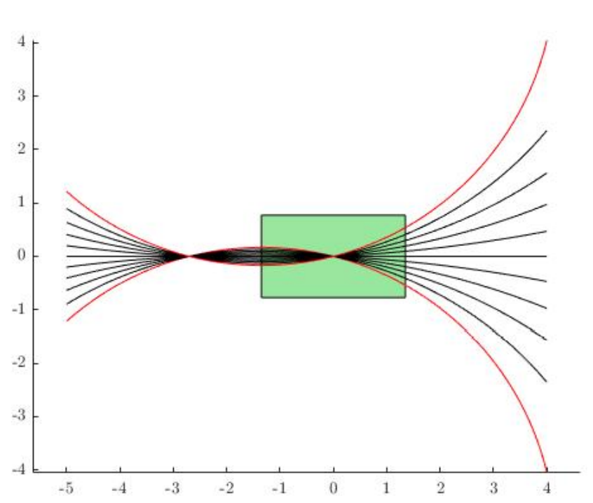
A Dynamically Consistent Distance Metric
Contact problem strikes again.
According to this metric, infinite distance if no contact is made!
What if there is no contact?
\begin{aligned}
\mathbf{B}^\mathrm{u} = 0
\end{aligned}
\begin{aligned}
\|f^\mathrm{u}({\color{red} q_0}, 0) - {\color{blue} q^\mathrm{u}_{goal}}\|^2_\mathbf{\Sigma^{-1}}
\end{aligned}
\begin{aligned}
\Sigma & = \mathbf{B}^\mathrm{u}{\mathbf{B}^\mathrm{u}}^\top
\end{aligned}
\begin{aligned}
d({\color{blue} q^\mathrm{u}_{goal}}; {\color{red} q_0}) =
\end{aligned}
Mahalanobis Distance induced by the Jacobian
\begin{aligned}
\mathbf{B}^\mathrm{u}\coloneqq \partial f^\mathrm{u}/\partial u
\end{aligned}
A Dynamically Consistent Distance Metric
Again, smoothing comes to the rescue!
\begin{aligned}
\|f^\mathrm{u}({\color{red} q_0}, 0) - {\color{blue} q^\mathrm{u}_{goal}}\|^2_\mathbf{\Sigma^{-1}}
\end{aligned}
\begin{aligned}
\Sigma & = \mathbf{B}^\mathrm{u}{\mathbf{B}^\mathrm{u}}^\top
\end{aligned}
\begin{aligned}
d({\color{blue} q^\mathrm{u}_{goal}}; {\color{red} q_0}) =
\end{aligned}
Mahalanobis Distance induced by the Jacobian
\begin{aligned}
\mathbf{B}^\mathrm{u}\coloneqq \partial f^\mathrm{u}/\partial u
\end{aligned}
A Dynamically Consistent Distance Metric
Now we can apply RRT to contact-rich systems!
A Dynamically Consistent Distance Metric
Now we can apply RRT to contact-rich systems!
However, these still require lots of random extensions!
A Dynamically Consistent Distance Metric
Now we can apply RRT to contact-rich systems!
However, these still require lots of random extensions!
With some chance, place the actuated object in a different configuration.
(Regrasping / Contact-Sampling)
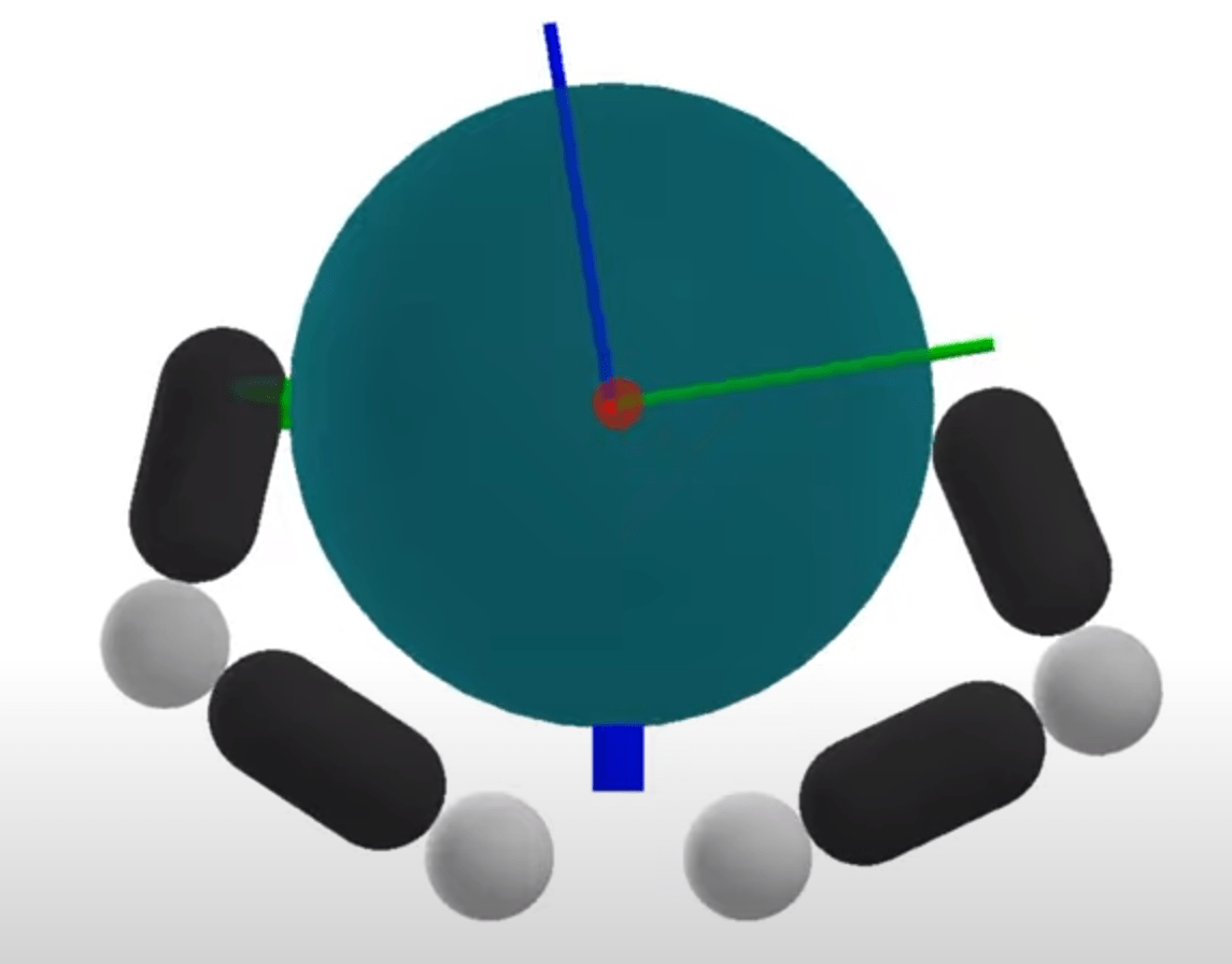
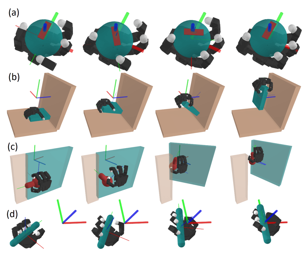
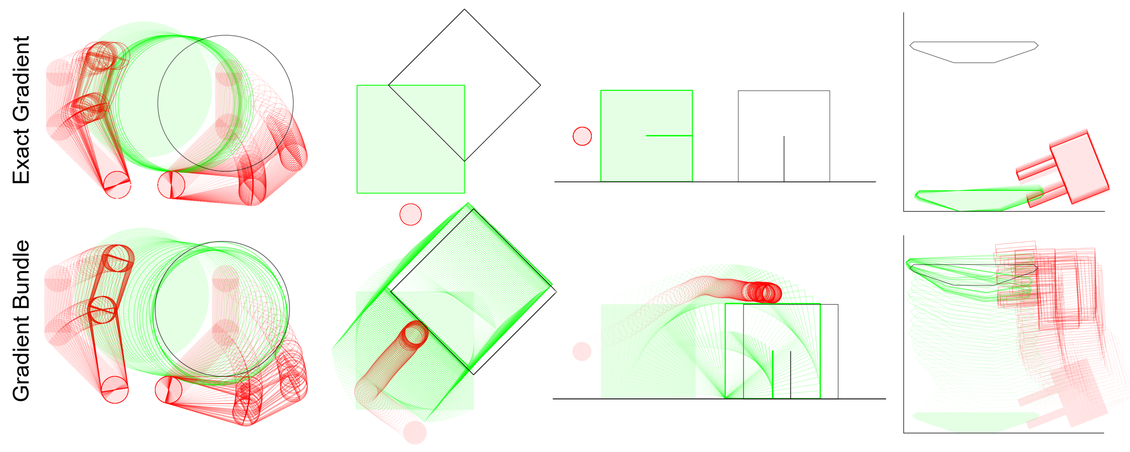
Contact-Rich RRT with Dynamic Smoothing
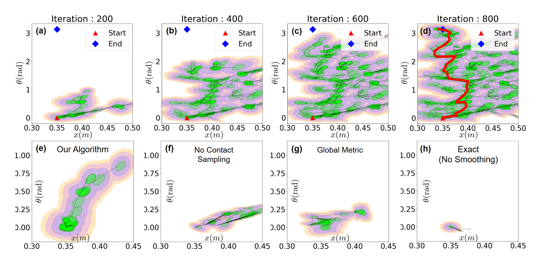
Our method can find solutions through contact-rich systems in few iterations! (~ 1 minute)
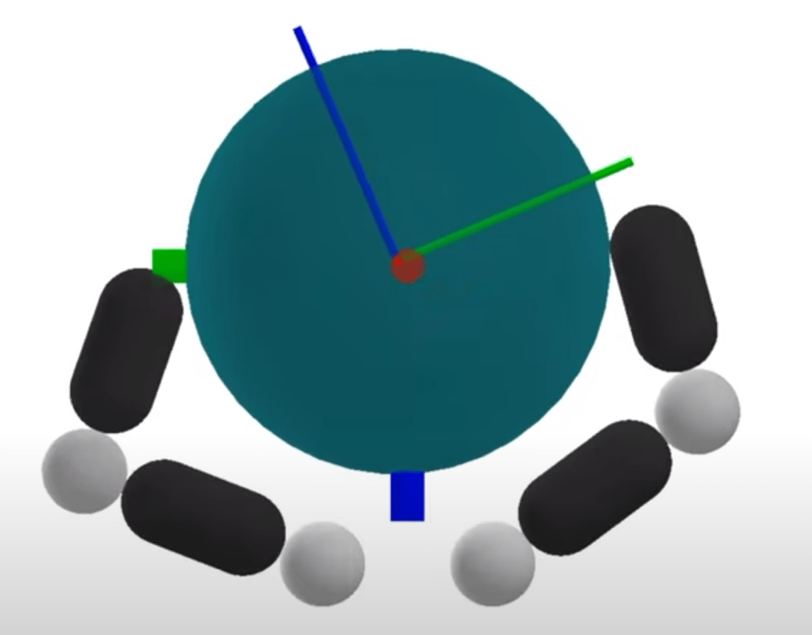
Contact-Rich RRT with Dynamic Smoothing
Without regrasping, the tree grows slowly.
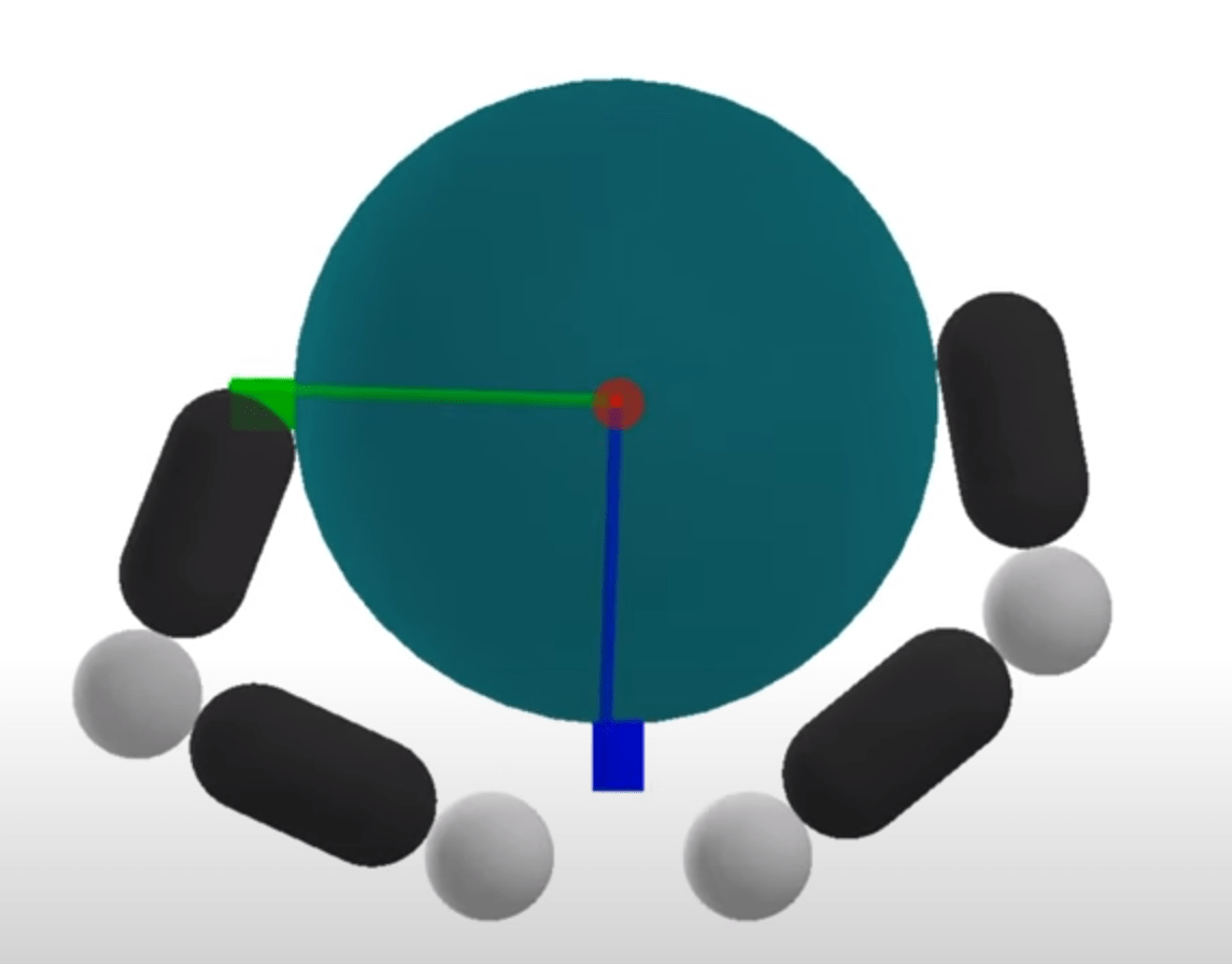
Contact-Rich RRT with Dynamic Smoothing
Using a global Euclidean metric hinders the growth of the tree.
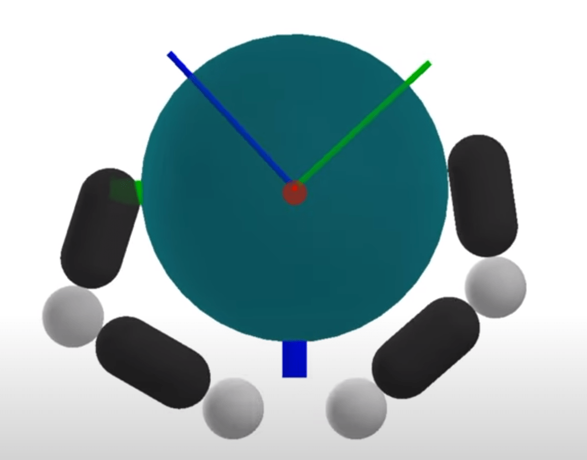
Contact-Rich RRT with Dynamic Smoothing
No dynamic smoothing gets completely stuck.
Efficient Global Planning for
Highly Contact-Rich Systems
Fast Solution Time
Beyond Local Solutions
Contact Scalability
RRT with Dynamics Smoothing
-
H.J. Terry Suh*, Tao Pang*, Russ Tedrake,
"Bundled Gradients through Contact via Randomized Smoothing",
RA-L 2022, Presented at ICRA 2022
-
H.J. Terry Suh, Max Simchowitz, Kaiqing Zhang, Russ Tedrake,
"Do Differentiable Simulators Give Better Policy Gradients?",
ICML 2022, Outstanding Paper Award
- Tao Pang*, H.J. Terry Suh*, Lujie Yang, Russ Tedrake,
"Global Planning for Contact-Rich Manipulation via Local Smoothing of Quasidynamic Contact Models",
TRO 2023, To be presented at ICRA 2024
Thank You
Smoothing Techniques for Non-Smooth Problems
Some non-smooth problems are successfully tackled by smooth approximations without sacrificing much from bias.
Is contact one of these problems?
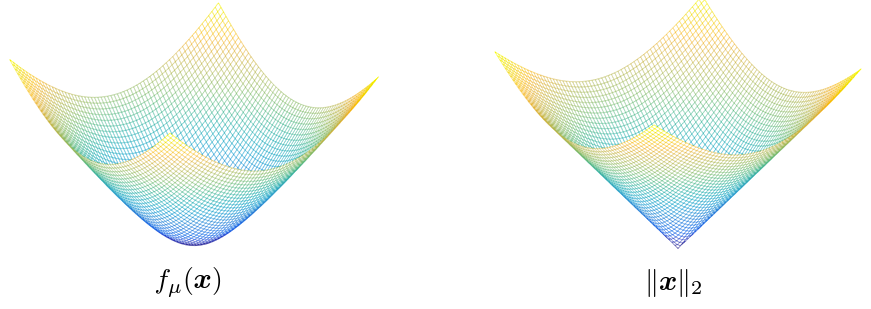
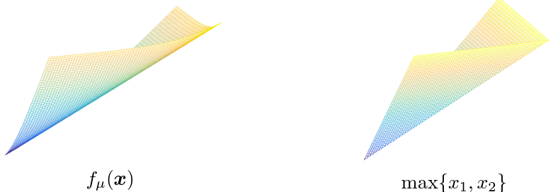
*Figures taken from Yuxin Chen's slides on "Smoothing for Non-smooth Optimization"
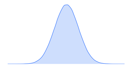
Smoothing in Optimization
We can formally define smoothing as a process of convolution with a smooth kernel,
f(x)
f_\rho(x)\coloneqq \mathbb{E}_{w\sim\rho }f(x + w)
In addition, for purposes of optimization, we are interested in methods that provide easy access to the derivative of the smooth surrogate.
Original Function
Smooth Surrogate
Derivative of the Smooth Surrogate:
\frac{\partial}{\partial x} f_\rho(x) = \frac{\partial}{\partial x} \mathbb{E}_{w\sim\rho }f(x + w)
These provide linearization Jacobians in the setting when f is dynamics, and policy gradients in the setting when f is a value function.
Taxonomy of Smoothing
Case 1. Analytic Smoothing
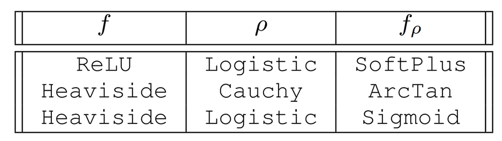
f_\rho(x)\coloneqq \mathbb{E}_{w\sim\rho }f(x + w)
- If the original function f and the distribution rho is sufficiently structured, we can also evaluate the smooth surrogate in closed form by computing the integral.
- This can be analytically differentiated to give the derivative.
- Commonly used in ML as smooth nonlinearities.
Taxonomy of Smoothing
Case 2. Randomized Smoothing, First Order
\begin{aligned}
f_\rho(x) & \coloneqq \mathbb{E}_{w\sim\rho }f(x + w) \\
& = \textstyle\frac{1}{N}\sum^N_{i=1} f(x + w_i)
\end{aligned}
- When we write convolution as an expectation, it motivates Monte-Carlo sampling methods that can estimate the value of the smooth surrogate.
- In order to obtain the derivative, we can use the Leibniz integral rule to exchange the expectation and the derivative.
- This means we can sample derivatives to approximate the derivative of the sampled function.
- Requires access to the derivative of the original function f.
- Also known as the Reparametrization (RP) gradient.
\begin{aligned}
\frac{\partial}{\partial x} f_\rho(x) & = \frac{\partial}{\partial x} \mathbb{E}_{w\sim\rho }f(x + w) = \mathbb{E}_{w\sim\rho}\left[\frac{\partial}{\partial x} f(x+w)\right] \\
& \approx \frac{1}{N} \sum^N_{i=1} \frac{\partial}{\partial x}f(x+w_i)
\end{aligned}
Taxonomy of Smoothing
Case 2. Randomized Smoothing, First Order
*Figures taken from John Duchi's slides on Randomized Smoothing
Taxonomy of Smoothing
Case 2. Randomized Smoothing, Zeroth-Order
\begin{aligned}
f_\rho(x) & \coloneqq \mathbb{E}_{w\sim\rho }f(x + w) \\
& = \textstyle\frac{1}{N}\sum^N_{i=1} f(x + w_i)
\end{aligned}
- Interestingly, we can obtain the derivative of the randomized smoothing objective WITHOUT having access to the gradients of f.
- This gradient is derived from Stein's lemma
- Known by many names: Likelihood Ratio gradient, Score Function gradient, REINFORCE gradient.
\begin{aligned}
\frac{\partial}{\partial x}\mathbb{E}_{w\sim\rho}[f(x+w)] = \mathbb{E}_{w\sim\rho}\left[f(x + w)S(w)^\top\right]
\end{aligned}
S(w) = \nabla_w \log \rho(w) = -\frac{\nabla \rho(w)}{\rho(w)}
This seems like it came out of nowhere? How can this be true?
Taxonomy of Smoothing
Rethinking Linearization as a Minimizer.
\min_{\mathbf{J},\mu} \frac{1}{2}\mathbb{E}_{w\sim\rho}\left[\|f(\bar{x} + w) - \mathbf{J}w - \mu\|^2_2\right]
- The linearization of a function provides the best linear model (i.e. up to first order) to approximate the function locally.
- We could use the same principle for a stochastic function.
- Fix a point xbar. If we were to sample bunch of f(xbar + w_i) and run a least-squares procedure to find the best linear model, this converges to the linearization of the smooth surrogate.
\begin{aligned}
\mathbf{J}^* & = \mathbb{E}_{w\sim \rho}\left[f(\bar{x} + w)w^\top\right]\mathbf{\Sigma}^{-1} \\
\mu^* & = \mathbb{E}_{w\sim\rho}\left[f(\bar{x} + w)\right]
\end{aligned}
Also provides a convenient way to compute the gradient in zeroth-order. Just sample and run least-squares!
Tradeoffs between structure and performance.
The generally accepted wisdom: more structure gives more performance.
Analytic smoothing
Randomized Smoothing
First-Order
Randomized Smoothing
Zeroth-Order
- Requires closed-form evaluation of the integral.
- No sampling required.
- Requires access to first-order oracle (derivative of f).
- Generally less variance than zeroth-order.
- Only requires zeroth-order oracle (value of f)
- High variance.
Structure Requirements
Performance / Efficiency
Smoothing of Optimal Control Problems
Optimal Control thorugh Non-smooth Dynamics
\begin{aligned}
\min_{\theta} & \; \bigg[V(\theta) = c_T(x_T) + \sum^{T-1}_{t=0} \gamma^t c(x_t, u_t)\bigg] \\
\text{s.t.} & \; x_{t+1} = f(x_t, u_t) \\
& \; u_t = \pi(x_t, \theta)
\end{aligned}
\begin{aligned}
\min_{\theta} & \; \bigg[V(\theta) = c_T(x_T) + \sum^{T-1}_{t=0} \gamma^t c(x_t, u_t)\bigg] \\
\text{s.t.} & \; {\color{red} x_{t+1} = \mathbb{E}_{w,v}\left[f(x_t + w_t, u_t+v_t)\right]} \\
& \; u_t = \pi(x_t, \theta)
\end{aligned}
Policy Optimization
Cumulative Cost
Dynamics
Policy (can be open-loop)
Dynamics Smoothing
\begin{aligned}
\min_\theta V(\theta)
\end{aligned}
Value Smoothing
\begin{aligned}
\min_{\theta} & \; {\color{red}\mathbb{E}_{w}}\bigg[V(\theta + w) = c_T(x_T) + \sum^{T-1}_{t=0} \gamma^t c(x_t, u_t)\bigg] \\
\text{s.t.} & \; x_{t+1} = f(x_t, u_t) \\
& \; {\color{red} u_t = \pi(x_t, \theta + w)}
\end{aligned}
Smoothing of Optimal Control Problems
\begin{aligned}
\min_{\theta} & \; \bigg[V(\theta) = c_T(x_T) + \sum^{T-1}_{t=0} \gamma^t c(x_t, u_t)\bigg] \\
\text{s.t.} & \; {\color{red} x_{t+1} = \mathbb{E}_{w,v}\left[f(x_t + w_t, u_t+v_t)\right]} \\
& \; u_t = \pi(x_t, \theta)
\end{aligned}
Dynamics Smoothing
What does it mean to smooth contact dynamics stochastically?
Since some samples make contact and others do not, averaging these "discrete modes" creates force from a distance.
Smoothing of Optimal Control Problems
\begin{aligned}
\min_{x_t,u_t} & \; \bigg[V(u_t) = c_T(x_T) + \sum^{T-1}_{t=0} \gamma^t c(x_t, u_t)\bigg] \\
\text{s.t.} & \; {\color{red} x_{t+1} = \mathbb{E}_{w,v}\left[f(x_t + w_t, u_t+v_t)\right]} \\
\end{aligned}
Dynamics Smoothing
\begin{aligned}
\min_{x_t, u_t} & \; \bigg[V(u_t) = x_T^\top \mathbf{Q}_T x_T + \sum^{T-1}_{t=0} \gamma^t \left[x_t^\top \mathbf{Q} x_t + u_t^\top \mathbf{R} u_t\right]\bigg] \\
\text{s.t.} & \; x_{t+1} = \mathbf{A}_t x_t + \mathbf{B}_t u_t + c_t \\
\end{aligned}
Quadratic Programming
To numerically solve this problem, we rely on the fact that we have a known dynamic programming solution to linear dynamics with quadratic cost.
Until convergence:
- Rollout current iterate of input sequence.
- Linearize dynamics around the trajectory
- Solve for the optimal input under linearized dynamics
Sequential Quadratic Programming
Sequential Quadratic Programming
Importantly, the linearization utilizes stochastic gradient estimation techniques.
Optimal Control with Dynamics Smoothing
Exact
Smoothed
Smoothing of Value Functions.
Optimal Control thorugh Non-smooth Dynamics
\begin{aligned}
\min_{\theta} & \; \bigg[V(\theta) = c_T(x_T) + \sum^{T-1}_{t=0} \gamma^t c(x_t, u_t)\bigg] \\
\text{s.t.} & \; x_{t+1} = f(x_t, u_t) \\
& \; u_t = \pi(x_t, \theta)
\end{aligned}
\begin{aligned}
\min_{\theta} & \; \bigg[V(\theta) = c_T(x_T) + \sum^{T-1}_{t=0} \gamma^t c(x_t, u_t)\bigg] \\
\text{s.t.} & \; {\color{red} x_{t+1} = \mathbb{E}_{w,v}\left[f(x_t + w_t, u_t+v_t)\right]} \\
& \; u_t = \pi(x_t, \theta)
\end{aligned}
Policy Optimization
Cumulative Cost
Dynamics
Policy (can be open-loop)
Dynamics Smoothing
\begin{aligned}
\min_\theta V(\theta)
\end{aligned}
Value Smoothing
\begin{aligned}
\min_{\theta} & \; {\color{red}\mathbb{E}_{w}}\bigg[V(\theta + w) = c_T(x_T) + \sum^{T-1}_{t=0} \gamma^t c(x_t, u_t)\bigg] \\
\text{s.t.} & \; x_{t+1} = f(x_t, u_t) \\
& \; {\color{red} u_t = \pi(x_t, \theta + w)}
\end{aligned}
f(x)
f_\rho(x)\coloneqq \mathbb{E}_{w\sim\rho }f(x + w)
Recall that smoothing turns into .
Why not just smooth the value function directly and run policy optimization?
Smoothing of Value Functions.
Original Problem
\begin{aligned}
\min_\theta V(\theta)
\end{aligned}
Long-horizon problems involving contact can have terrible landscapes.
Smoothing of Value Functions.
Smooth Surrogate
\begin{aligned}
\min_\theta \mathbb{E}_w V(\theta + w)
\end{aligned}
The benefits of smoothing are much more pronounced in the value smoothing case.
Beautiful story - noise sometimes regularizes the problem, developing into helpful bias.
How do we take gradients of smoothed value function?
Analytic smoothing
Randomized Smoothing
First-Order
Randomized Smoothing
Zeroth-Order
- Requires differentiability over dynamics, reward, policy.
- Generally lower variance.
- Only requires zeroth-order oracle (value of f)
- High variance.
Structure Requirements
Performance / Efficiency
Pretty much not possible.
How do we take gradients of smoothed value function?
First-Order Policy Search with Differentiable Simulation
Policy Gradient Methods in RL (REINFORCE / TRPO / PPO)
- Requires differentiability over dynamics, reward, policy.
- Generally lower variance.
- Only requires zeroth-order oracle (value of f)
- High variance.
Structure Requirements
Performance / Efficiency
Turns out there is an important question hidden here regarding the utility of differentiable simulators.
Do Differentiable Simulators Give Better Policy Gradients?
Very important question for RL, as it promises lower variance, faster convergence rates, and more sample efficiency.
What do we mean by "better"?
Consider a simple stochastic optimization problem
\min_\theta F(\theta) = \min_\theta \mathbb{E}_{w\sim\mathcal{N}(w;0,\sigma^2)} f(\theta + w)
First-Order Gradient Estimator
\begin{aligned}
\nabla_\theta \mathbb{E}_w f(\theta + w) & = \mathbb{E}_w f(\theta + w) \\
& = \frac{1}{N}\sum^N_{i=1}\nabla_\theta f(\theta + w_i)
\end{aligned}
Zeroth-Order Gradient Estimator
\begin{aligned}
\nabla_\theta \mathbb{E}_w f(\theta + w) & = \frac{1}{\sigma^2}\mathbb{E}_w [f(\theta + w)w] \\
& = \frac{1}{N}\sum^N_{i=1}\frac{1}{\sigma^2} f(\theta + w_i)w_i
\end{aligned}
Then, we can define two different gradient estimators.
What do we mean by "better"?
First-Order Gradient Estimator
\begin{aligned}
\nabla_\theta \mathbb{E}_w f(\theta + w) & = \mathbb{E}_w f(\theta + w) \\
& = \frac{1}{N}\sum^N_{i=1}\nabla_\theta f(\theta + w_i)
\end{aligned}
Zeroth-Order Gradient Estimator
\begin{aligned}
\nabla_\theta \mathbb{E}_w f(\theta + w) & = \frac{1}{\sigma^2}\mathbb{E}_w [f(\theta + w)w] \\
& = \frac{1}{N}\sum^N_{i=1}\frac{1}{\sigma^2} f(\theta + w_i)w_i
\end{aligned}
Bias
Variance
Common lesson from stochastic optimization:
1. Both are unbiased under sufficient regularity conditions
2. First-order generally has less variance than zeroth order.
What happens in Contact-Rich Scenarios?
Bias
Variance
Common lesson from stochastic optimization:
1. Both are unbiased under sufficient regularity conditions
2. First-order generally has less variance than zeroth order.
Bias
Variance
Bias
Variance
We show two cases where the commonly accepted wisdom is not true.
1st Pathology: First-Order Estimators CAN be biased.
2nd Pathology: First-Order Estimators can have MORE
variance than zeroth-order.
Bias from Discontinuities
1st Pathology: First-Order Estimators CAN be biased.
\begin{aligned}
\nabla_\theta \mathbb{E}_w f(\theta + w) & = \mathbb{E}_w f(\theta + w) = \frac{1}{N}\sum^N_{i=1}\nabla_\theta f(\theta + w_i)
\end{aligned}
What's worse: the empirical variance is also zero!
(The estimator is absolutely sure about an estimate that is wrong)
Not just a pathology, could happen quite often in contact.
Empirical Bias leads to High Variance
Perhaps it's a modeling artifact? Contact can be softened.
- From a low-sample regime, no statistical way to distinguish between an actual discontinuity and a very stiff function.
- Generally, stiff relaxations lead to high variance. As relaxation converges to true discontinuity, variance blows up to infinity, and suddenly turns into bias!
- Zeroth-order escapes by always thinking about the cumulative effect over some finite interval.
Variance of First-Order Estimators
2nd Pathology: First-order Estimators CAN have more variance than zeroth-order ones.
\begin{aligned}
\textbf{Var}_\theta\left[{\color{blue}\frac{1}{N}\frac{1}{\sigma^2}\sum^N_{i=1}f(\theta + w_i)w_i}\right] \leq \frac{\dim \theta}{N\sigma^2}\max_w\|f(\theta + w)\|^2_2
\end{aligned}
\begin{aligned}
\textbf{Var}_\theta\left[{\color{red}\frac{1}{N}\sum^N_{i=1}\nabla_\theta f(\theta + w_i)}\right] \leq \frac{1}{N}\max_w \|\nabla_\theta f(\theta + w)\|^2_2
\end{aligned}
Scales with Gradient
Scales with Function Value
Scales with dimension of decision variables.
High-Variance Events
Case 1. Persistent Stiffness
Case 2. Chaotic
- Contact modeling using penalty method is a bad idea for differentiable policy search
- Gradients always has the spring stiffness value!
- High variance depending on initial condition
- Zeroth-order always bounded in value, but the gradients can be very high.
Motivating Contact-rich RRT
How do we overcome local minima of local gradient-based methods?
Our ideal solution
The RRT Algorithm
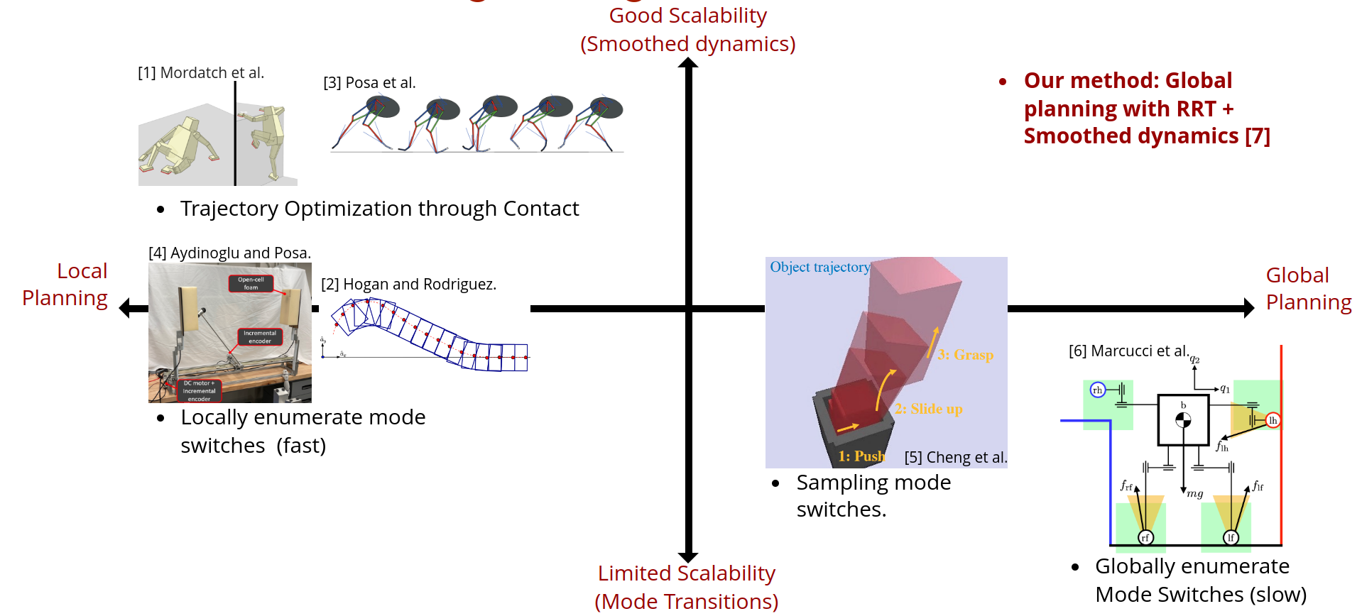
Global Search with Smoothing: Contact-Rich RRT
Motivating Contact-Rich RRT
Sampling-Based Motion Planning is a popular solution in robotics for complex non-convex motion planning
How do we define notions of nearest?
How do we extend (steer)?
- Nearest states in Euclidean space are not necessarily reachable according to system dynamics (Dubin's car)
- Typically, kinodynamic RRT solves trajopt
- Potentially a bit costly.
Reachability-Consistent Distance Metric
Reachability-based Mahalanobis Distance

d(q;\bar{q})
How do we come up with a distance metric between q and qbar in a dynamically consistent manner?
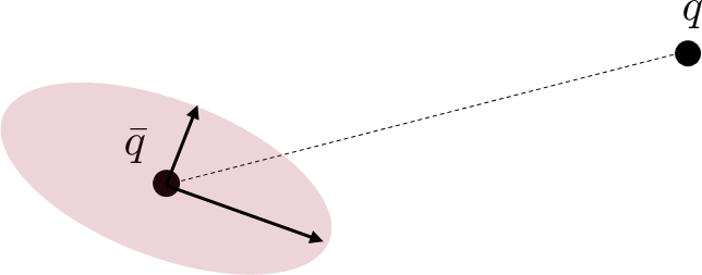
Reachability-Consistent Distance Metric
Reachability-based Mahalanobis Distance
How do we come up with a distance metric between q and qbar in a dynamically consistent manner?
q_+ = \mathbf{B}(\bar{q},\bar{u})\delta u + f(\bar{q},\bar{u})
Consider a one-step input linearization of the system.
Then we could consider a "reachability ellipsoid" under this linearized dynamics,
\mathcal{E} = \{q_+ | q_+ = \mathbf{B}(\bar{q},\bar{u})\delta u + f(\bar{q},\bar{u}), \|\delta u \| \leq 1\}
Note: For quasidynamic formulations, ubar is a position command, which we set as the actuated part of qbar.
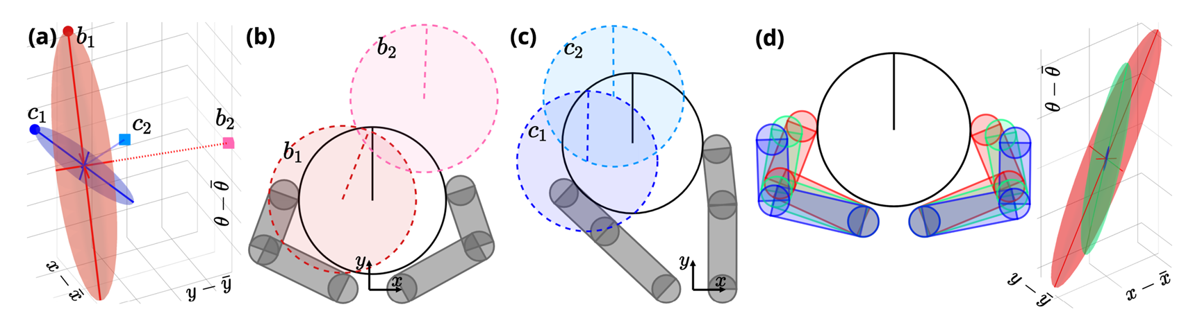
Reachability Ellipsoid
Reachability Ellipsoid
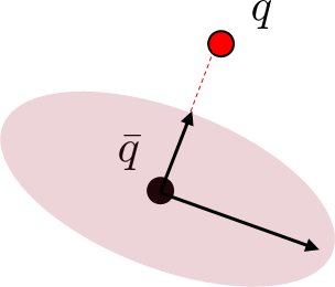
\mathcal{E} = \{q_+ | q_+ = \mathbf{B}(\bar{q},\bar{u})\delta u + f(\bar{q},\bar{u}), \|\delta u \| \leq 1\}
Intuitively, if B lengthens the direction towards q from a uniform ball, q is easier to reach.
On the other hand, if B decreases the direction towards q, q is hard to reach.
Mahalanobis Distance of an Ellipsoid
Reachability Ellipsoid
\mathcal{E} = \{q_+ | q_+ = \mathbf{B}(\bar{q},\bar{u})\delta u + f(\bar{q},\bar{u}), \|\delta u \| \leq 1\}
The B matrix induces a natural quadratic form for an ellipsoid,
\begin{aligned}
d_\gamma(q;\bar{q}) & \coloneqq \frac{1}{2}(q-\mu)^\top \mathbf{\Sigma}_\gamma^{-1}(q - \mu) \\
\mathbf{\Sigma}_\gamma & \coloneqq \mathbf{B}(\bar{q},\bar{u})\mathbf{B}(\bar{q},\bar{u})^\top + \gamma\mathbf{I}_n \\
\mu & \coloneqq f(\bar{q},\bar{u})
\end{aligned}
Mahalanobis Distance using 1-Step Reachability
Note: if BBT is not invertible, we need to regularize to property define a quadratic distance metric numerically.
Smoothed Distance Metric
\begin{aligned}
d_{{\color{red}\rho},\gamma}(q;\bar{q}) & \coloneqq \frac{1}{2}(q-\mu)^\top \mathbf{\Sigma}_{{\color{red}\rho},\gamma}^{-1}(q - \mu) \\
\mathbf{\Sigma}_\gamma & \coloneqq \mathbf{B}_{\color{red}\rho}(\bar{q},\bar{u})\mathbf{B}_{\color{red}\rho}(\bar{q},\bar{u})^\top + \gamma\mathbf{I}_n \\
\mu & \coloneqq f_{\color{red}\rho}(\bar{q},\bar{u})
\end{aligned}
For Contact:
Don't use the exact linearization, but the smooth linearization.
Global Search with Smoothing
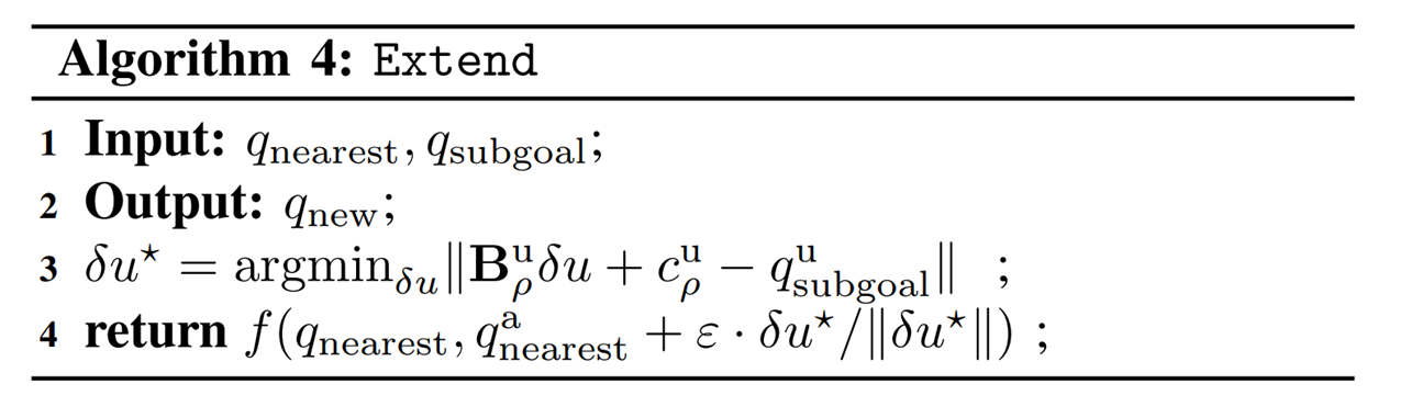
Dynamically consistent extension
Theoretically, it is possible to use long-horizon trajopt algorithms such as iLQR / DDP.
Here we simply do one-step trajopt and solve least-squares.
Importantly, the actuation matrix for least-squares is smoothed, but we rollout the actual dynamics with the found action.
Dynamically consistent extension
Contact Sampling
With some probability, we execute a regrasp (sample another valid contact configuration) in order to encourage further exploration.

Global Search with Smoothing
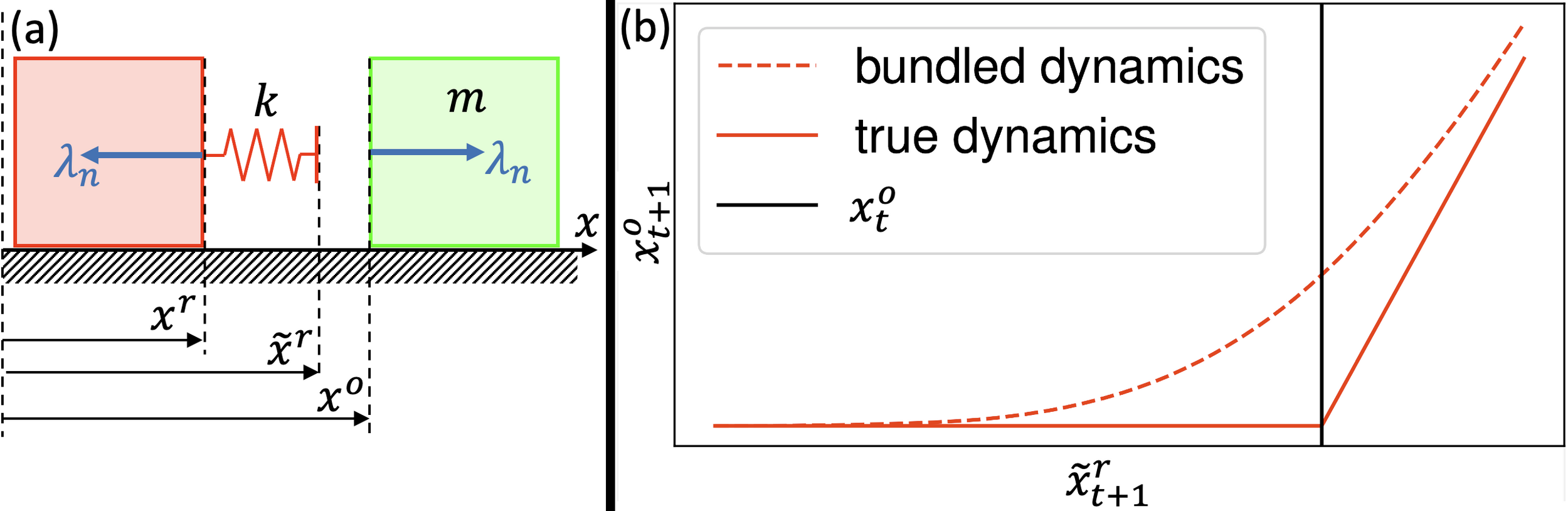
Smoothing of Contact Dynamics
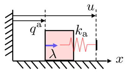
Without going too much into details of multibody contact dynamics, we will use time-stepping, quasidynamic formulation of contact.
- We assume that velocities die out instantly
- Inputs to the system are defined by position commands to actuated bodies.
- The actuated body and the commanded position is connected through an impedance source k.
\begin{aligned}
\text{find} \quad & \delta q \\
\text{s.t.} \quad & hk(q + \delta q - u) = \lambda \\
& 0 \leq q + \delta q \perp \lambda \geq 0
\end{aligned}
Equations of Motion (KKT Conditions)
Non-penetration
(Primal feasibility)
Complementary slackness
Dual feasibility
Force Balance
(Stationarity)
\begin{aligned}
\min_{\delta q}\quad & \frac{1}{2} hk(\delta q)^2 - hk(u - q)\delta q \\
\text{s.t.} \quad & q + \delta q \geq 0
\end{aligned}
Quasistatic QP Dynamics
We can randomize smooth this with first order methods using sensitivity analysis or use zeroth-order randomized smoothing.
But can we smooth this analytically?
Barrier (Interior-Point) Smoothing
\begin{aligned}
\min_{\delta q}\quad & \frac{1}{2} hk(\delta q)^2 - hk(u - q)\delta q \\
\text{s.t.} \quad & q + \delta q \geq 0
\end{aligned}
Quasistatic QP Dynamics
\begin{aligned}
\text{find} \quad & \delta q \\
\text{s.t.} \quad & hk(q + \delta q - u) = \lambda \\
& 0 \leq q + \delta q \perp \lambda \geq 0
\end{aligned}
Equations of Motion (KKT Conditions)
\begin{aligned}
\min_{\delta q}\quad & \frac{1}{2} hk(\delta q)^2 - hk(u - q)\delta q - \frac{1}{\kappa}\log(q + \delta q)
\end{aligned}
Interior-Point Relaxation of the QP
Equations of Motion (Stationarity)
hk(q + \delta q - u) = \frac{1}{\kappa}\left(\frac{1}{q + \delta q}\right)
\lambda (q + \delta q) = \kappa^{-1}
Impulse
Relaxation of complementarity
"Force from a distance"
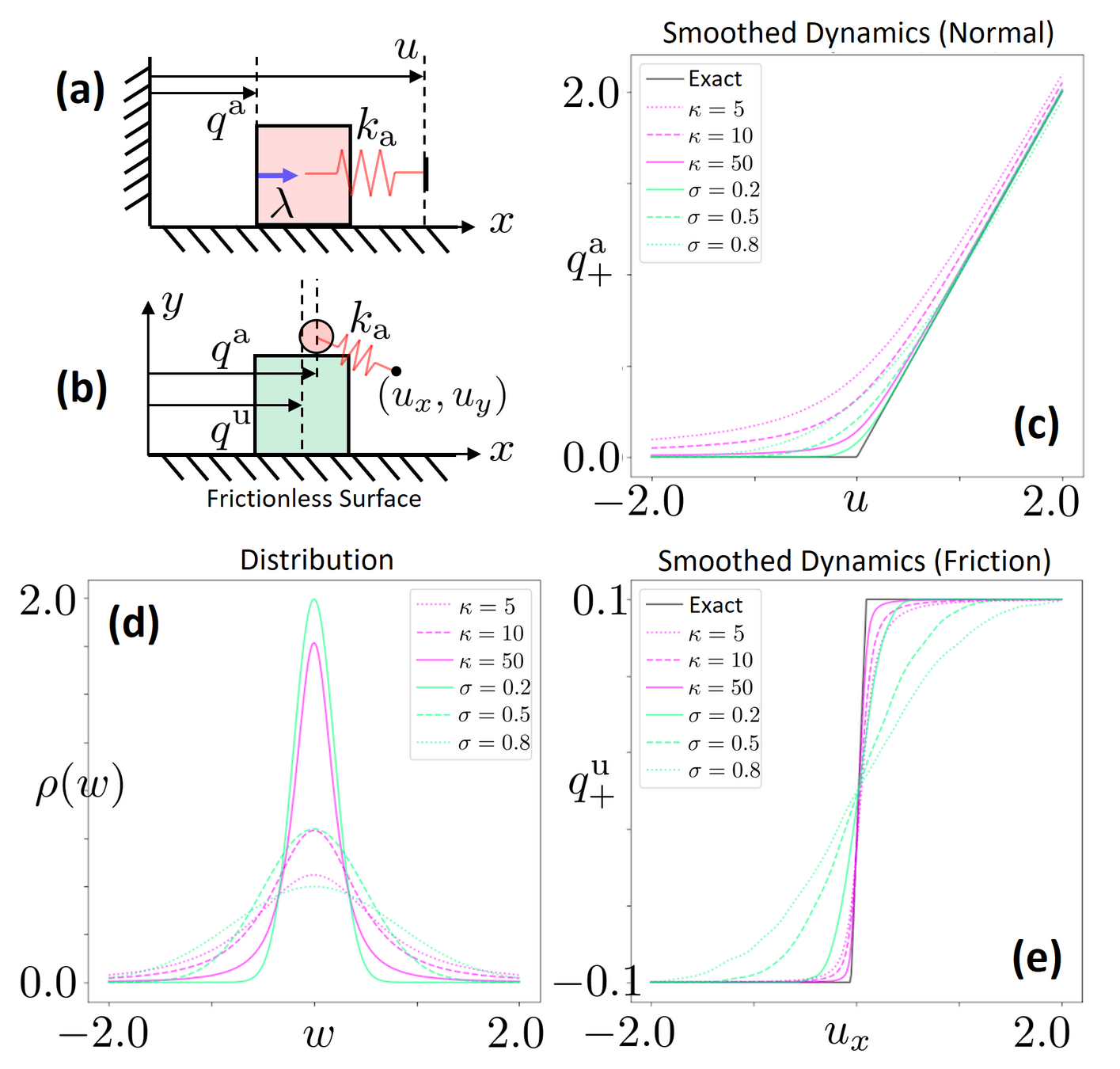
What does smoothing do to contact dynamics?

- Both schemes (randomized smoothing and barrier smoothing) provides "force from a distance effects" where the exerted force increases with distance.
- Provides gradient information from a distance.
- In contrast, without smoothing, zero gradients and flat landscapes cause problems for gradient-based optimization.
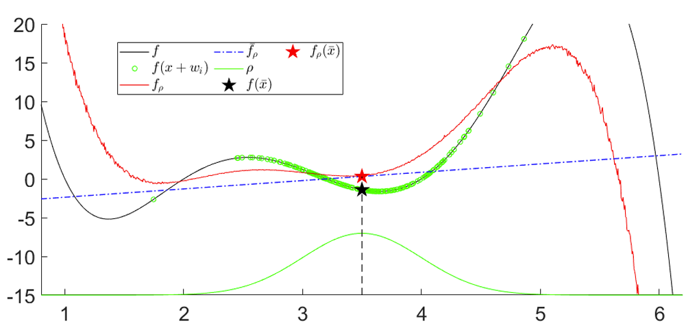
Is barrier smoothing a form of convolution?
Equivalence of Randomized and Barrier Smoothing.
- For the simple 1D pusher system, it turns out that one can show that barrier smoothing also implements a convolution with the original function and a kernel.
- This is an elliptical distribution with a "fatter tail" compared to a Gaussian".
\rho(w) = \sqrt{\frac{4 hk\kappa}{(w^\top 4h\kappa w + 4)^3}}
Later result shows that there always exists such a kernel for Linear Complementary Systems (LCS).
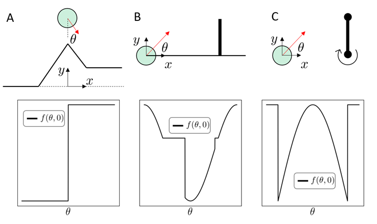
Limitations of Smoothing
Contact is non-smooth. But Is it truly "discrete"?
The core thesis of this talk:
The local decisions of where to make contact are better modeled as continuous decisions with some smooth approximations.
My viewpoint so far:
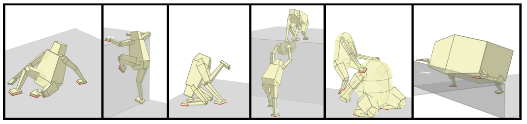
Limitations of Smoothing
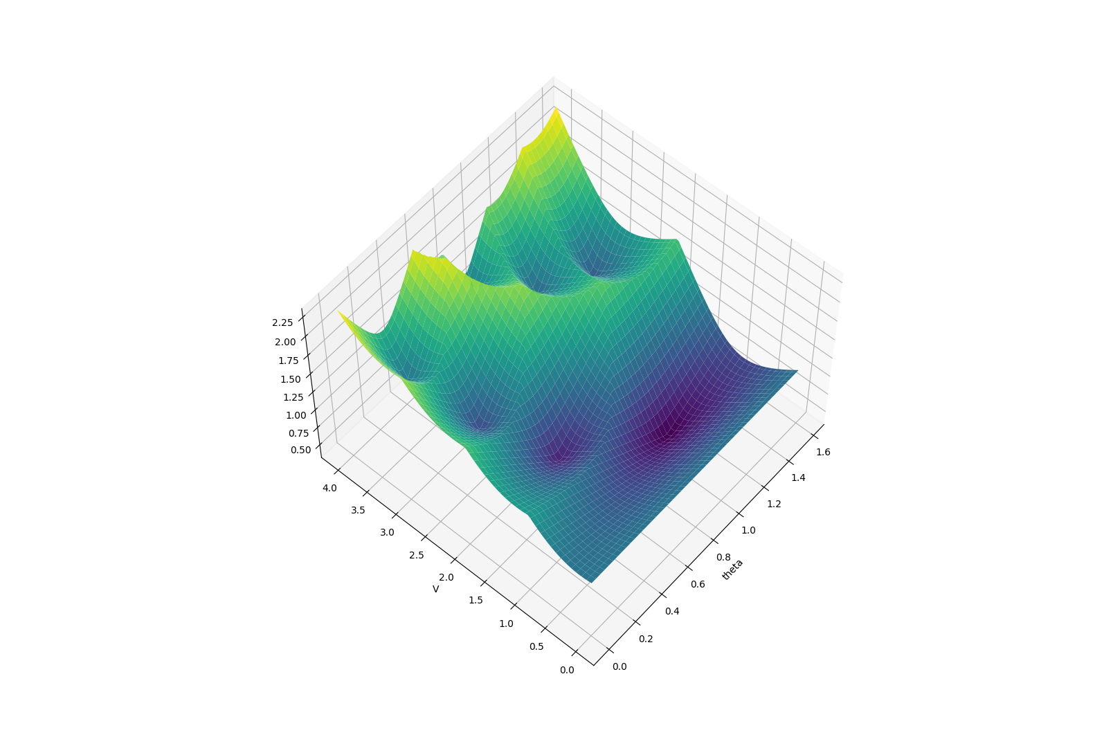
These reveal true discrete "modes" of the decision making process.
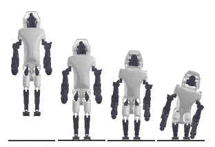
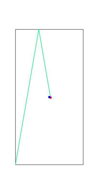
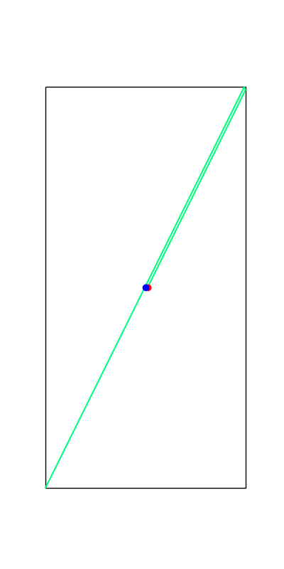
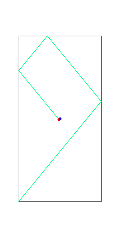
Limitations of Smoothing
\theta
Apply negative impulse
to stand up.
Apply positive impulse to bounce on the wall.
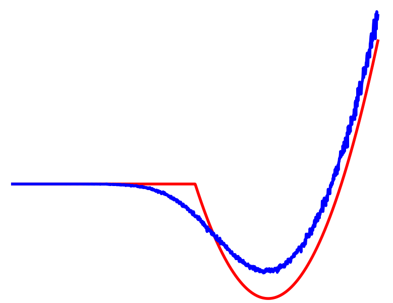
Bias of Smoothing
\begin{aligned}
\min_{u} \quad & \|q^u_\text{next} - q^u_g\|^2_\mathbf{Q} \\
\text{s.t.} \quad & q^u_\text{next} = {\color{red}\mathbf{B}^u_\rho}(q,\bar{u})(u - \bar{u}) + {\color{red}f^u_\rho}(q,\bar{u}) \\
& |u - \bar{u}| \leq \varepsilon\mathbf{1}
\end{aligned}
q^u
q^a
u
\lambda
\lambda
rho subscript denotes smoothing
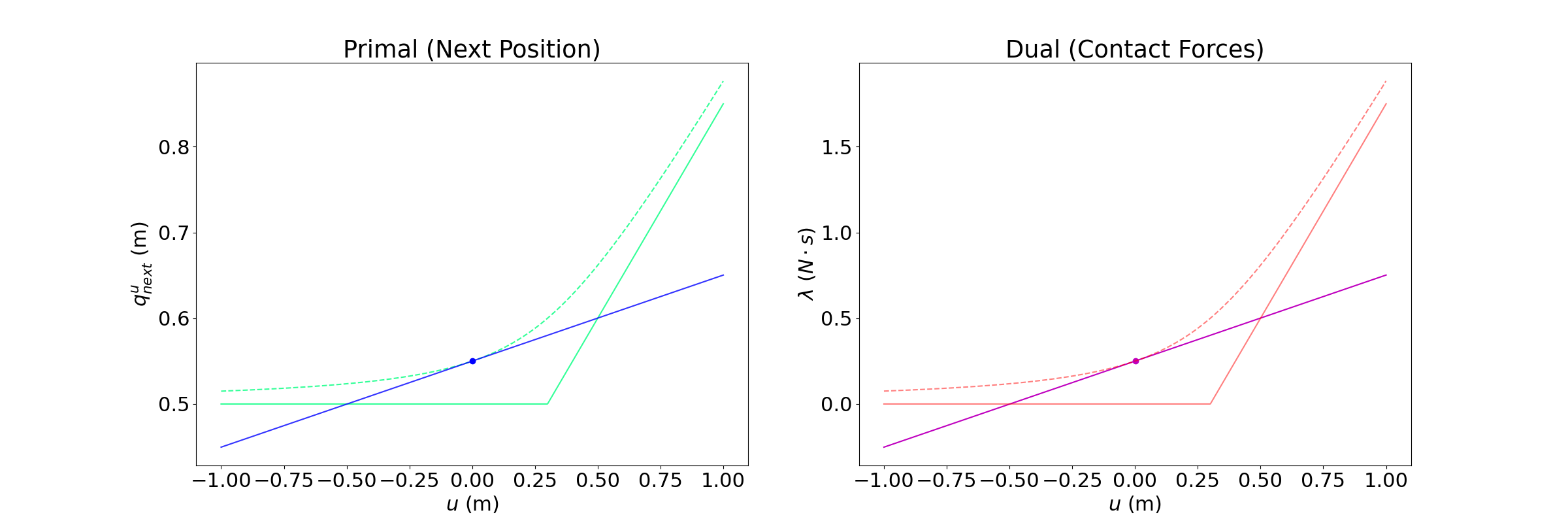
We have linearized the smoothened dynamics around u = qa.
Depending on where we set the goal to be, we see three distinct regions.
Bias of Smoothing
\begin{aligned}
\min_{u} \quad & \|q^u_\text{next} - q^u_g\|^2_\mathbf{Q} \\
\text{s.t.} \quad & q^u_\text{next} = {\color{red}\mathbf{B}^u_\rho}(q,\bar{u})(u - \bar{u}) + {\color{red}f^u_\rho}(q,\bar{u}) \\
& |u - \bar{u}| \leq \varepsilon\mathbf{1}
\end{aligned}
q^u
q^a
u
\lambda
\lambda
rho subscript denotes smoothing
0.5m
0.0m
Region 1. Beneficial Bias
Goal = 0.61m
Optimal input
The linearized model provides helpful bias, as the optimal input moves the actuated body towards making contact.
Bias of Smoothing
\begin{aligned}
\min_{u} \quad & \|q^u_\text{next} - q^u_g\|^2_\mathbf{Q} \\
\text{s.t.} \quad & q^u_\text{next} = {\color{red}\mathbf{B}^u_\rho}(q,\bar{u})(u - \bar{u}) + {\color{red}f^u_\rho}(q,\bar{u}) \\
& |u - \bar{u}| \leq \varepsilon\mathbf{1}
\end{aligned}
q^u
q^a
u
\lambda
\lambda
rho subscript denotes smoothing
0.5m
0.0m
Region 2. Hurtful Bias
Goal = 0.52m
Optimal input
If you command the actuated body to hold position, the unactuated body will be pushed away due to smoothing.
The actuated body wants to go backwards in order to decrease this effect if the goal is not too in front of the unactuated body.
Bias of Smoothing
\begin{aligned}
\min_{u} \quad & \|q^u_\text{next} - q^u_g\|^2_\mathbf{Q} \\
\text{s.t.} \quad & q^u_\text{next} = {\color{red}\mathbf{B}^u_\rho}(q,\bar{u})(u - \bar{u}) + {\color{red}f^u_\rho}(q,\bar{u}) \\
& |u - \bar{u}| \leq \varepsilon\mathbf{1}
\end{aligned}
q^u
q^a
u
\lambda
\lambda
rho subscript denotes smoothing
0.5m
0.0m
Region 3. Violation of unilateral contact
Goal = 0.45m
Optimal input
If you set the goal to behind the unactuated body, the linear model thinks that it can pull, and will move backwards.
Motivating Gradient Interpolation
Bias
Variance
Common lesson from stochastic optimization:
1. Both are unbiased under sufficient regularity conditions
2. First-order generally has less variance than zeroth order.
Bias
Variance
Bias
Variance
1st Pathology: First-Order Estimators CAN be biased.
2nd Pathology: First-Order Estimators can have MORE
variance than zeroth-order.
Can we automatically decide which of these categories we fall into based on statistical data?
The Alpha-Ordered Gradient Estimator
Perhaps we can do some interpolation of the two gradients based on some criteria.
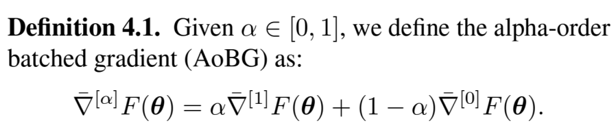
\min_{\alpha\in[0, 1]} \textbf{Var}(\bar{\nabla}^{[\alpha]}F(\theta)) = \alpha^2\hat{\sigma}^2_1 + (1-\alpha)^2 \hat{\sigma}_0^2
Previous works attempt to minimize the variance of the interpolated estimator using empirical variance.
Robust Interpolation
\min_{\alpha\in[0, 1]} \textbf{Var}(\bar{\nabla}^{[\alpha]}F(\theta)) = \alpha^2\hat{\sigma}^2_1 + (1-\alpha)^2 \hat{\sigma}_0^2
Thus, we propose a robust interpolation criteria that also restricts the bias of the interpolated estimator.
\begin{aligned}
\min_{\alpha\in[0, 1]} \; & \textbf{Var}(\bar{\nabla}^{[\alpha]}F(\theta)) \\
\text{s.t.} \; & \textbf{Bias}(\bar{\nabla}^{[\alpha]}F(\theta)) \leq \gamma
\end{aligned}
Robust Interpolation
Robust Interpolation
\begin{aligned}
\min_{\alpha\in[0, 1]} \; & \textbf{Var}(\bar{\nabla}^{[\alpha]}F(\theta)) \\
\text{s.t.} \; & \textbf{Bias}(\bar{\nabla}^{[\alpha]}F(\theta)) \leq \gamma
\end{aligned}
Implementation
\begin{aligned}
\min_{\alpha\in[0, 1]} \; & \alpha^2\hat{\sigma}_1^2 + (1 - \alpha)^2\hat{\sigma}^2_0 \\
\text{s.t.} \; & \varepsilon + \alpha\|\bar{\nabla}^{[1]}F - \bar{\nabla}^{[0]} F \| \leq \gamma
\end{aligned}
Confidence Interval on the zeroth-order gradient.
Difference between the gradients.
Key idea: Unit-test the first-order estimate against the unbiased zeroth-order estimate to guarantee correctness probabilistically. .
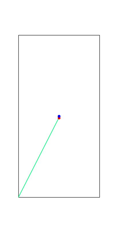
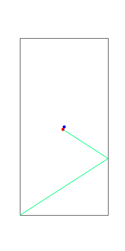
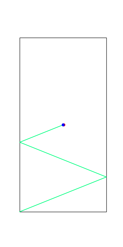
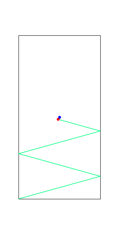
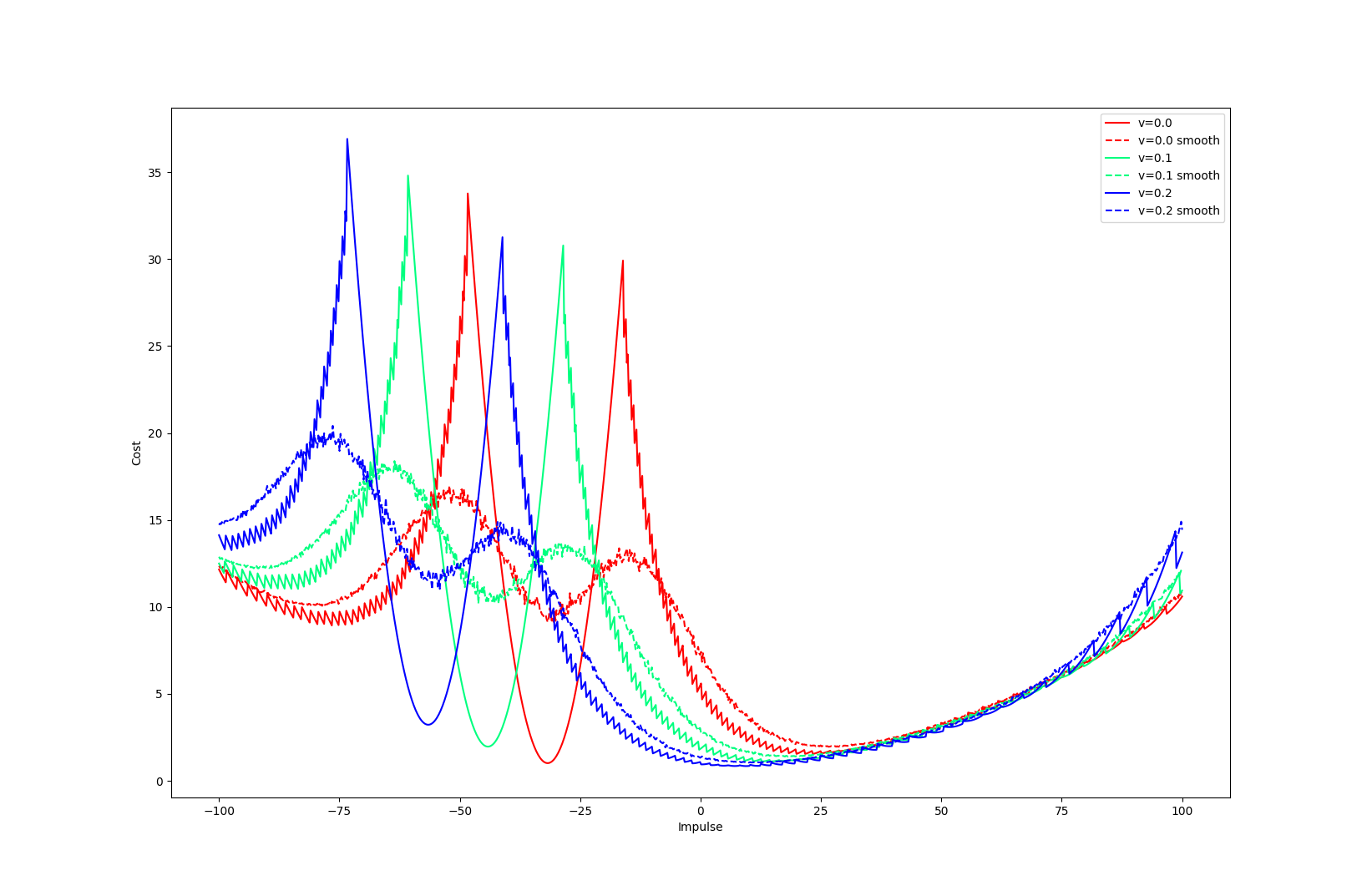
Results: Ball throwing on Wall
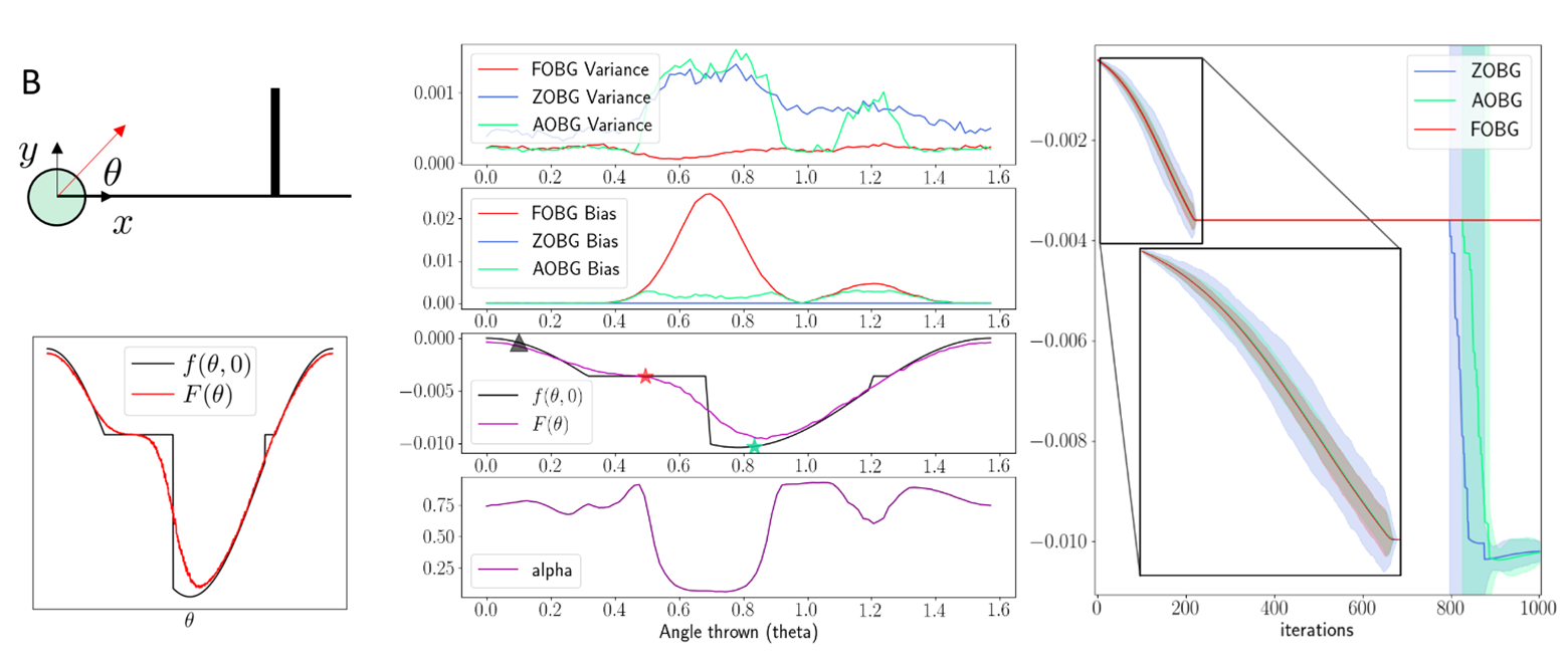
Key idea: Do not commit to zeroth or first uniformly,
but decide coordinate-wise which one to trust more.
Results: Policy Optimization
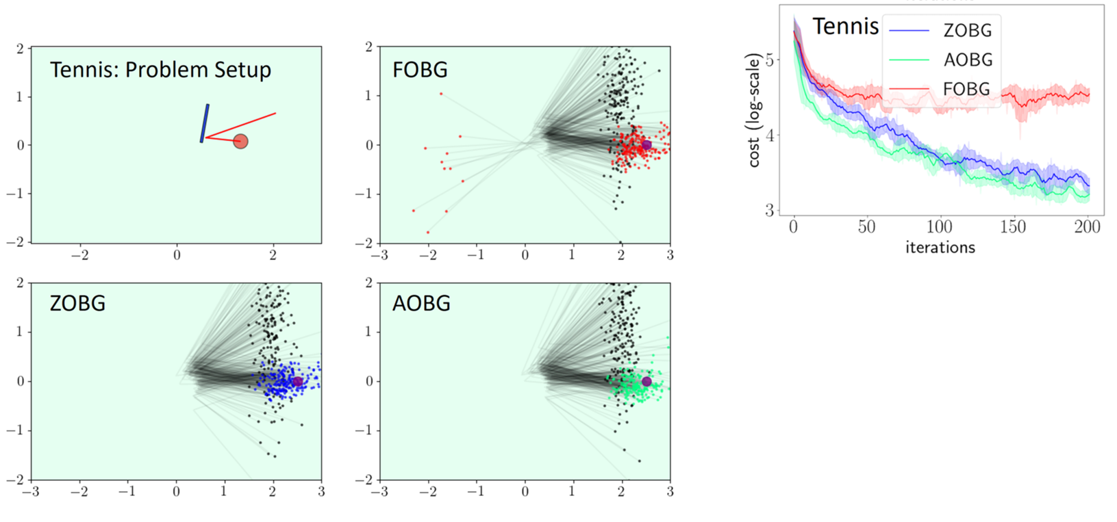
Able to capitalize on better convergence of first-order methods while being robust to their pitfalls.
KAIST Talk
By Terry Suh


