An Alternative to EM for Gaussian Mixture Models
Victor Sanches Portella
MLRG @ UBC
August 11, 2021
Why this paper?
Interesting application of Riemannian optimization to an important problem in ML
Details of the technicalities are not important
Yet, we have enough to sense the flavor of the field
Gaussian Mixture Models
Gaussian Mixture Models
A GMM is a convex combination of a fixed number of Gaussians
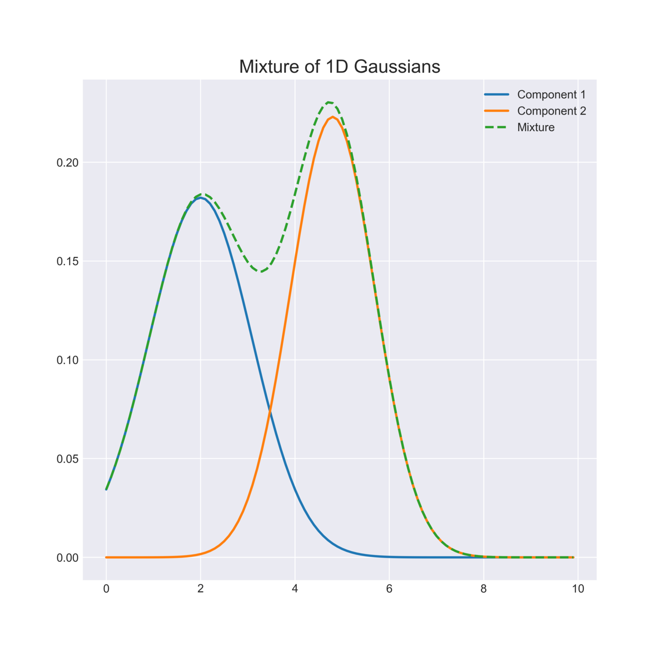
Image source: https://angusturner.github.io/assets/images/mixture.png
Gaussian Mixture Models
A GMM is a convex combination of a fixed number of Gaussians
Density of a \(K\)-mixture on \(\mathbb{R}^d\):
\displaystyle p(x) = \sum_{i = 1}^K \alpha_i \; p_{\mathcal{N}}(x; \mu_i, \Sigma_i)
Mean and Covariance of \(i\)-th Gaussian
Gaussian density
Weight of \(i\)-th Gaussian
(Must sum to 1)
Find GMM most likely to generate data points \(x_1, \dotsc, x_n \)
Fitting a GMM
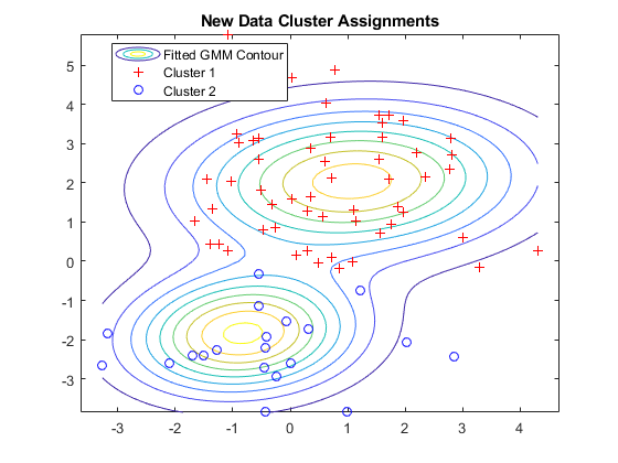
Image source: https://towardsdatascience.com/gaussian-mixture-models-d13a5e915c8e
Find GMM most likely to generate data points \(x_1, \dotsc, x_n \)
Fitting a GMM
Idea: use means \(\mu_i\) and covariances \(\Sigma_i\) that maximize log-likelihood
\displaystyle \max \sum_{i = 1}^n \log\Big(\sum_{j = 1}^K \alpha_i \; p_{\mathcal{N}}(x_i; \mu_j, \Sigma_j)\Big)
\displaystyle \sum_{i = 1}^n
\displaystyle x_i
\{
\alpha \in \Delta_n
\mu_j \in \mathbb{R}^d
\Sigma_j \succ 0
\Sigma_j \succ 0
Hard to describe
Open - No clear projection
Classical optimization methods (Newton, CG, IPM) struggle
Optimization vs "\(\succ 0\)"
Slowdown when iterates get closer to boundary
IPM works, but it is slow
Force positive definiteness via "Cholesky decomposition"
Adds spurious maxima/minima
\Sigma = L L^T
Slow
Expectation Maximization guarantees \(\succ 0\) "for free"
Easy for GMM's
Fast in practice
EM: Iterative method to find (local) max-likely parameters
EM in one slide
E-step: Fix parameters, find "weighted log-likelihood"
M-step: Find parameters by maximizing the "weighted log-likelihood"
For GMM's:
E-step: Given \(\mu_i, \Sigma_i\), compute \(P(x_j \in \mathcal{N}_i)\)
M-step: Max weighted log-likelihood with weights \(P(x_j \in \mathcal{N}_i)\)
\(= p(x_j ; \mu_i, \Sigma_i)\)
CLOSED FORM SOLUTION FOR GMMs!
Guarantees \(\succ 0\) for free
Riemannian Optimization
Manifold of PD Matrices
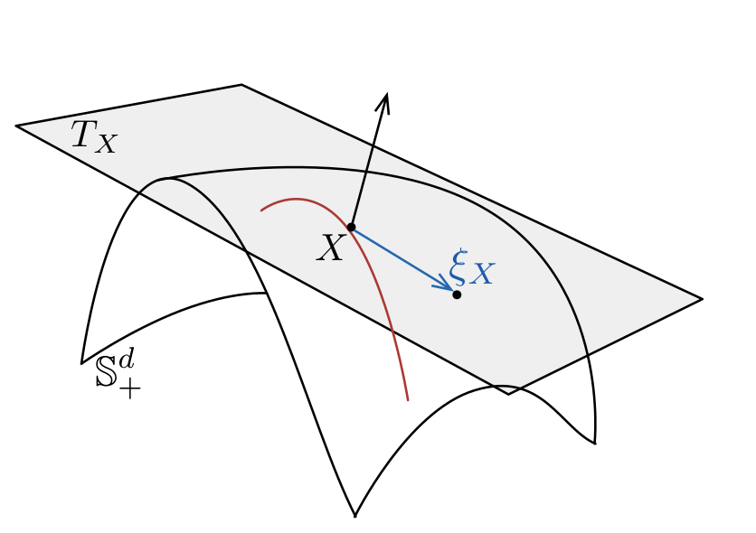
Manifold of PD Matrices
\mathbb{P}^d = \{\Sigma \in \mathbb{R}^{d \times d} \colon \Sigma \succ 0\}
Rimennian metric at
\Sigma
\langle X,Y \rangle_{\Sigma} = \mathrm{Tr}(\Sigma^{-1} X \Sigma^{-1} Y)
\Sigma
Tangent space at a point
T_{\Sigma}
\equiv
All symmetric matrices
Remark: Blows up when \(\Sigma\) is close to the boundary
Optimization Structure
General steps:
1 - Find descent direction
2 - Perform line-search and step with retraction
Retraction: a way to move on a manifold along a tangent direction
\mathrm{Ret}_{\Sigma} \colon T_{\Sigma} \to \mathbb{P}^d
\mathrm{Ret}_{\Sigma}(0) = \Sigma
\mathrm{D Ret}_{\Sigma}(0) = \mathrm{Id}
\{
Not necessarily follows a geodesic!
\mathrm{D}
In this paper, we will only use the Exponential Map:
\mathrm{Ret}_{\Sigma}(D) = \gamma_D(1)
where
\gamma_D(t)
is the geodesic starting at \(\Sigma\) with direction \(D\)
The Exponential Map
\mathrm{Ret}_{\Sigma}(D) = \gamma_D(1)
where
\(\gamma_D(t)\) is the geodesic starting at \(\Sigma\) with direction \(D\)
Geodesic between \(\Sigma\) and \(\Gamma\)
\(\Sigma\) at \(t = 0\) and \(\Gamma\) at \(t = 1\)
\Sigma^{\frac{1}{2}} (\Sigma^{-\frac{1}{2}} \Gamma \Sigma^{-\frac{1}{2}})^t \Sigma^{\frac{1}{2}}
\displaystyle (
\displaystyle )^{}
{}^t
From this (?), we get the form of the exponential map
\mathrm{Ret}_{\Sigma}(D) = \Sigma^{\frac{1}{2}} \exp(\Sigma^{-\frac{1}{2}} D \Sigma^{-\frac{1}{2}}) \Sigma^{\frac{1}{2}}
= \Sigma \; \exp(\Sigma^{-1} D )
Gradient Descent
GD on the Riemannian Manifold \(\mathbb{P}^d\):
\Sigma_{t+1} = \mathrm{Ret}_{\Sigma_t}( - \eta_t \; \mathrm{grad} f(\Sigma_t) )
\mathrm{grad} f(\Sigma_t)
\mathrm{grad} f(\Sigma_t)
\equiv
Riemannian gradient of \(f\).
Depends on the metric!
\displaystyle =
\frac{1}{2} \Sigma_t \Big(\nabla f(\Sigma_t) + \nabla f(\Sigma_t)^T \Big) \Sigma_t
If we have time, we shall see conditions for convergence of SGD
The methods the authors use are Conjugate Gradient and LBFGS.
x_{t+1} = x_t - \eta_t \nabla f(x_t)
Traditional gradient descent (GD):
Defining those depends on the idea of vector transport and Hessians. I'll skip these descriptions
Riemannian opt for GMMs
We have a geometric structure on \(\mathbb{P}^d\). The other variable can stay in the traditional Euclidean space.
We can apply methods for Riemannian optimization!
... but they are way slower than traditional EM
GMMs and Geodesic Convexity
Single Gaussian Estimation
Maximum Likelihood estimation for a single Gaussian:
\displaystyle \max_{\mu, \; \Sigma \succ 0} \mathcal{L}(\mu, \Sigma) \coloneqq \sum_{i = 1}^n \log p_{\mathcal{N}}(x_i; \mu, \Sigma)
\(\mathcal{L}\) is concave!
In fact, the above has a closed form solution
In a Riemannian manifold, meaning of convexity changes
Geodesic convexity (g-convexity):
f(\gamma(t)) \leq (1 - t) f(\Sigma_1) + t f(\Sigma_2)
\gamma(t)
Geodesic from \(\Sigma_1\) to \(\Sigma_2\)
\(\mathcal{L}\) is not g-concave
Single Gaussian Estimation
Maximum Likelihood estimation for a single Gaussian:
\displaystyle \max_{\mu, \; \Sigma \succ 0} \mathcal{L}(\mu, \Sigma) \coloneqq \sum_{i = 1}^n \log p_{\mathcal{N}}(x_i; \mu, \Sigma)
\(\mathcal{L}\) is concave!
\(\mathcal{L}\) is not g-concave
Solution: lift the function to a higher dimension!
\displaystyle \max_{S \succ 0} \hat{\mathcal{L}}(S) \coloneqq \sum_{i = 1}^n \log q_{\mathcal{N}}(y_i; S)
\displaystyle =
\begin{pmatrix}
x_i \\ 1
\end{pmatrix}
(d + 1) \times (d+1)
\(\hat{\mathcal{L}}\) is g-concave
\displaystyle =
c \cdot p_{\mathcal{N}}(y_i; 0, S)
Single Gaussian Estimation
\displaystyle \max_{\mu, \; \Sigma \succ 0} \mathcal{L}(\mu, \Sigma) \coloneqq \sum_{i = 1}^n \log p_{\mathcal{N}}(x_i; \mu, \Sigma)
\displaystyle \max_{S \succ 0} \hat{\mathcal{L}}(S) \coloneqq \sum_{i = 1}^n \log q_{\mathcal{N}}(y_i; S)
Theorem If \(\mu^*, \Sigma^*\) max \(\mathcal{L}\) and \(S^*\) maxs \(\hat{\mathcal{L}}\), then
\(\mathcal{L}\) is not g-concave
\(\hat{\mathcal{L}}\) is g-concave
\displaystyle \mathcal{L}(\mu^*, \Sigma^*) = \hat{\mathcal{L}}(S^*)
S^* =
\begin{pmatrix}
\Sigma^* + \mu^* {\mu^{*}}^T & \mu^* \\
\mu^* & 1
\end{pmatrix}
and
Theorem If \(\mu^*, \Sigma^*\) max \(\mathcal{L}\) and \(S^*\) maxs \(\hat{\mathcal{L}}\), then
\displaystyle \mathcal{L}(\mu^*, \Sigma^*) = \hat{\mathcal{L}}(S^*)
S^* =
\begin{pmatrix}
\Sigma^* + \mu^* {\mu^{*}}^T & \mu^* \\
\mu^* & 1
\end{pmatrix}
and
Proof idea:
S =
\begin{pmatrix}
\Sigma + s \mu {\mu}^T & s \mu \\
s \mu & s
\end{pmatrix}
s > 0
Write
Optimal choice of \(s\) is 1 \(\implies\) both \(\mathcal{L}\) and \(\hat{\mathcal{L}}\) agree
PS: \(\Sigma^* \succ 0\) by Shur's complement Lemma
Back to Many Gaussians
\displaystyle \max \mathcal{L}\big(\{\mu_j\}, \{\Sigma_j\} \big) = \sum_{i = 1}^n \log\Big(\sum_{j = 1}^K \alpha_i \; p_{\mathcal{N}}(x_i; \mu_j, \Sigma_j)\Big)
For now, fix
\alpha_1, \dotsc, \alpha_k
\displaystyle \max \hat{\mathcal{L}}\big(\{S_j\} \big) = \sum_{i = 1}^n \log\Big(\sum_{j = 1}^K \alpha_i \; q_{\mathcal{N}}(y_i; S_j)\Big)
Theorem The local maxima of \(\mathcal{L}\) and of \(\hat{\mathcal{L}}\) agree
What about \(\alpha_1, \dotsc, \alpha_K\)? Reparameterize to use unconstrained opt
\displaystyle \alpha_j \coloneqq \frac{\exp(w_j)}{\sum_{k = 1}^K \exp(w_k)}
I think there are not many guarantees on final \(\alpha_j\)'s
Plots!
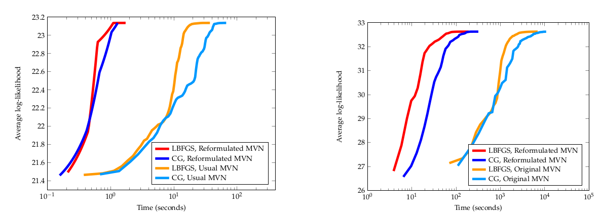
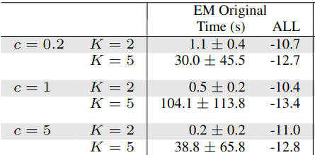
The effect of the lifting on convergence
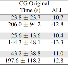
Plots!
EM vs Riemannian Opt
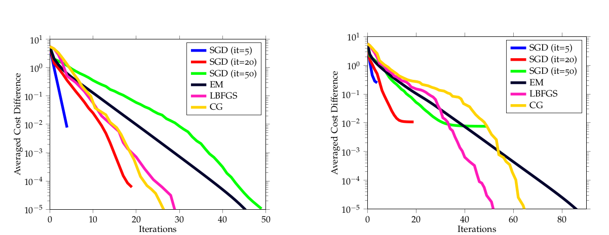
K = 3
K = 7
PS: Reformulation helps Cholesky as well, but this information disappeared from the final version
Remarks on What I Skipped
Step-size Line Search
Lifting with Regularization
Details on vector transport and 2nd order methods
Riemannian SGD
Riemannian SGD
x_{t+1} = \mathrm{Ret}_{x_t}\big(- \eta_t \; \mathrm{grad} f_{i_t}(x_t)\big),
\(i_t\) a random index
Assumptions on \(f\):
Riemann Lip. Smooth
f\big(\mathrm{Ret}_{x}(d)\big) \leq f(x) + \langle \mathrm{grad} f(x), d \rangle + \frac{L}{2} ||d ||^2
Unbiased Gradients
\mathbb{E}[ \mathrm{grad} f_{i_t}(x) - \mathrm{grad} f(x)] = 0
Bounded Variance
\mathbb{E}\big[ ||\mathrm{grad} f_{i_t}(x) - \mathrm{grad} f(x)||^2\big] \leq \sigma
We want to minimize
f = \frac{1}{n} \sum_{i = 1}^n f_i
Riemannian Stochastic Gradient Descent:
Riemannian SGD
x_{t+1} = \mathrm{Ret}_{x_t}\big(- \eta_t \; \mathrm{grad} f_{i_t}(x_t)\big)
Assumptions on \(f\):
Riemann Lip. Smooth
Unbiased Gradients
Bounded Variance
f = \frac{1}{n} \sum_{i = 1}^n f_i
Riemannian SGD
Theorem If one of the following holds:
i) Bounded gradients:
|| \mathrm{grad} f(x)|| \leq G \quad \forall i
ii) Outputs an uniformly random iterate
Then
\displaystyle \mathbb E \Big[ || \mathrm{grad} f(x_{\tau})||^2 \Big] \leq O\Bigg(\frac{1}{\sqrt{T}}\Bigg),
\(\tau\) is unif. random if (ii)
\(\tau\) is best iter. if (i)
(No need for bdd var)
Does SGD work for GMM?
Do the conditions for SGD to converge hold for GMMs?
Theorem If \(\eta_t \leq 1\), then iterates stay in a compact set.
(For some reason they analyze SGD with a different retraction...)
Remark Objective function is not Riemannian Lip. smooth outside of a compact set
Fact Iterates stay in a compact set \(\implies\)
Bounded Gradients
\(\implies\)
Classical Lip. smoothness
\(\implies\)
Thm from Riemannian Geometry
Riemann Lip. smoothness
It works!
With a different retraction and at a slower rate...?
MLRG - Riemannian opt
By Victor Sanches Portella


