




Erik Jansson
WASP and KAW postdoctoral fellow in the Cambridge Image Analysis Group and CRA at Wolfson College.
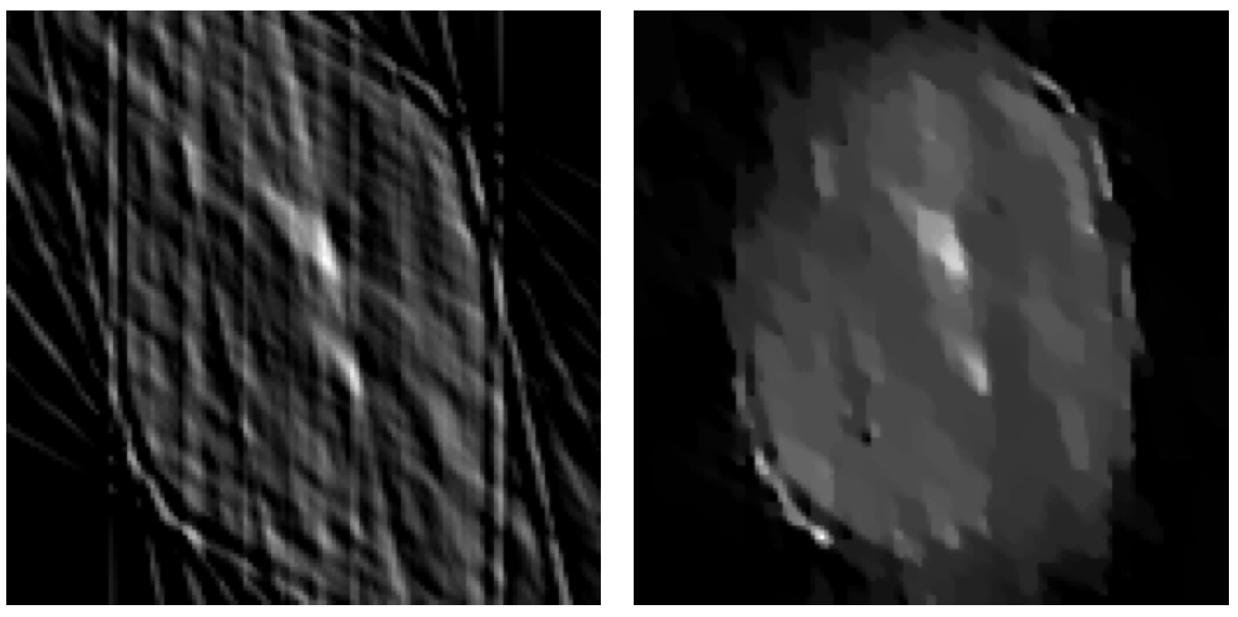
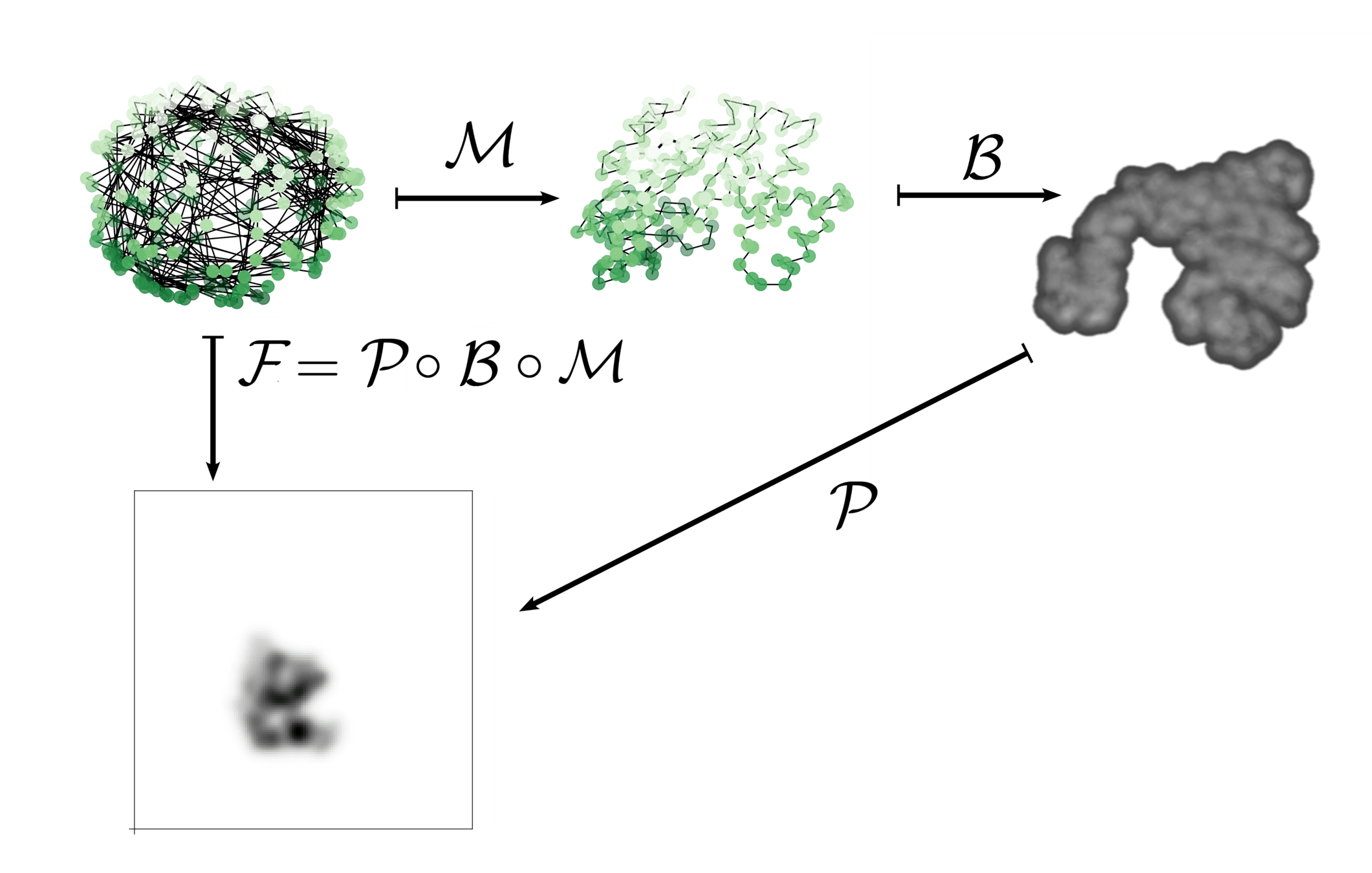
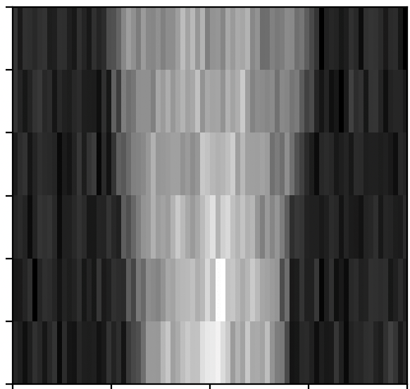
Sinogram (observation)
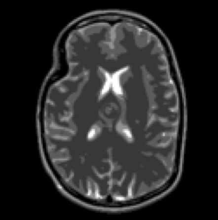
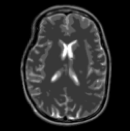
Reconstruction by deformation
Template
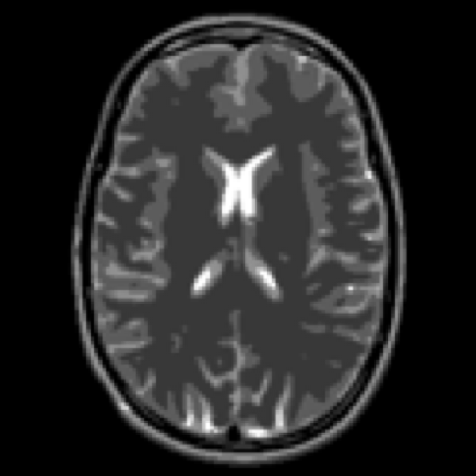
Target
Other name: matching problems
Provides one possible approach
But what is a shape?
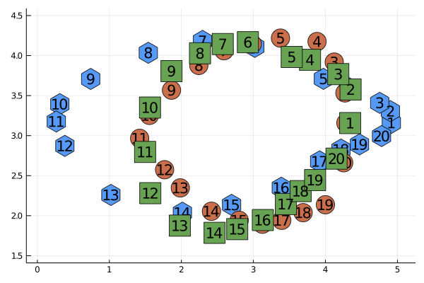
Point cloud
Smooth function
Density
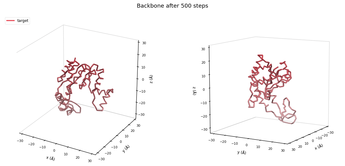
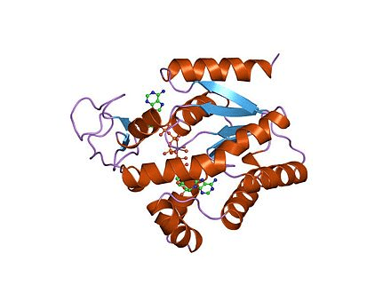
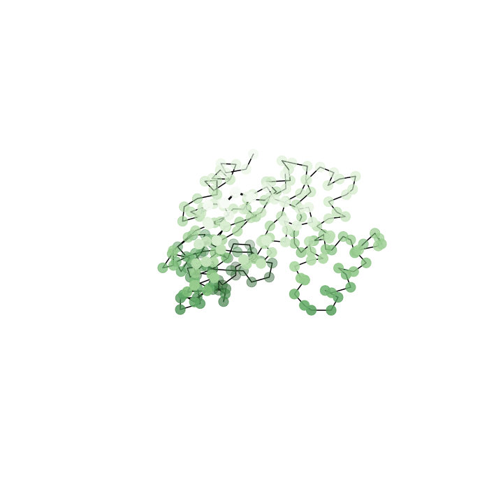
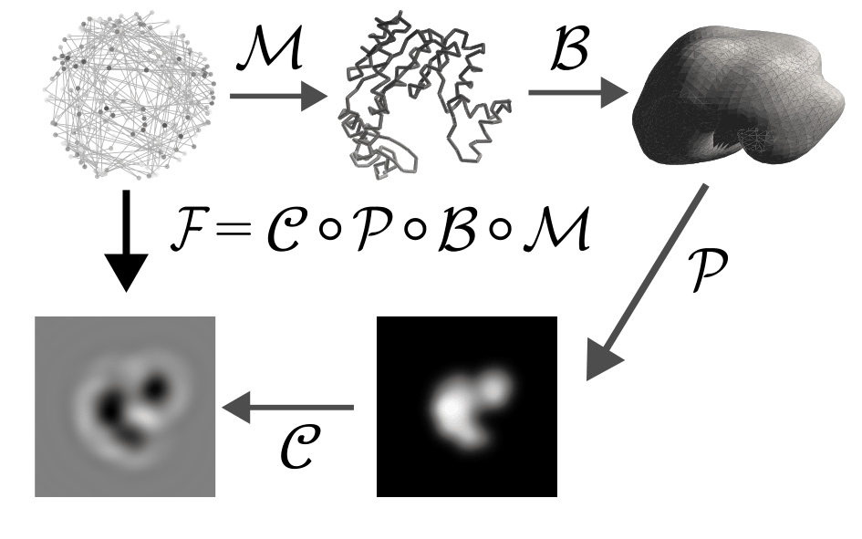
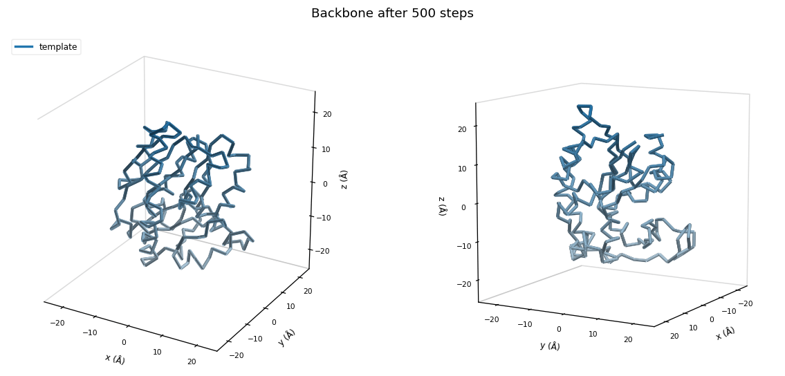
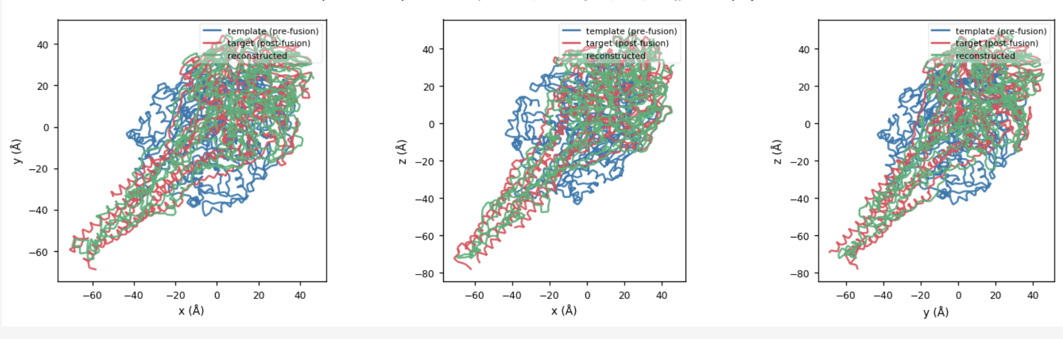
Protein backbones
But what is a shape?
Image from brain scan
A shape is an element of a shape space
A shape space is a space acted on by a suitable Lie group \(G\)
So what's a shape space?
So what's a Lie group?
So what's a Lie group?
Need to know: set of transformations that can be composed and inverted
Examples:
Shapes are in a (metric) space \(V\) acted upon by a Lie group of deformations \(G\).
Find the group element \(\gamma \in G\) minimizing the energy:
Goal is to find the optimal group element taking
\(v\)
\(w\)
to (or close to)
Simple example:
\(v\)
\(w\)
\(w\)
\(v\)
\(gv\)
Optimal solution: rotate until aligned
of a shape space
\(v,w\)
\(V\)
Lie Group
\(G\)
acts on elements
Classic case: \(G = \operatorname{Diff}(M)\), \(V = C^\infty(M)\)
All spaces involved are infinite-dimensional
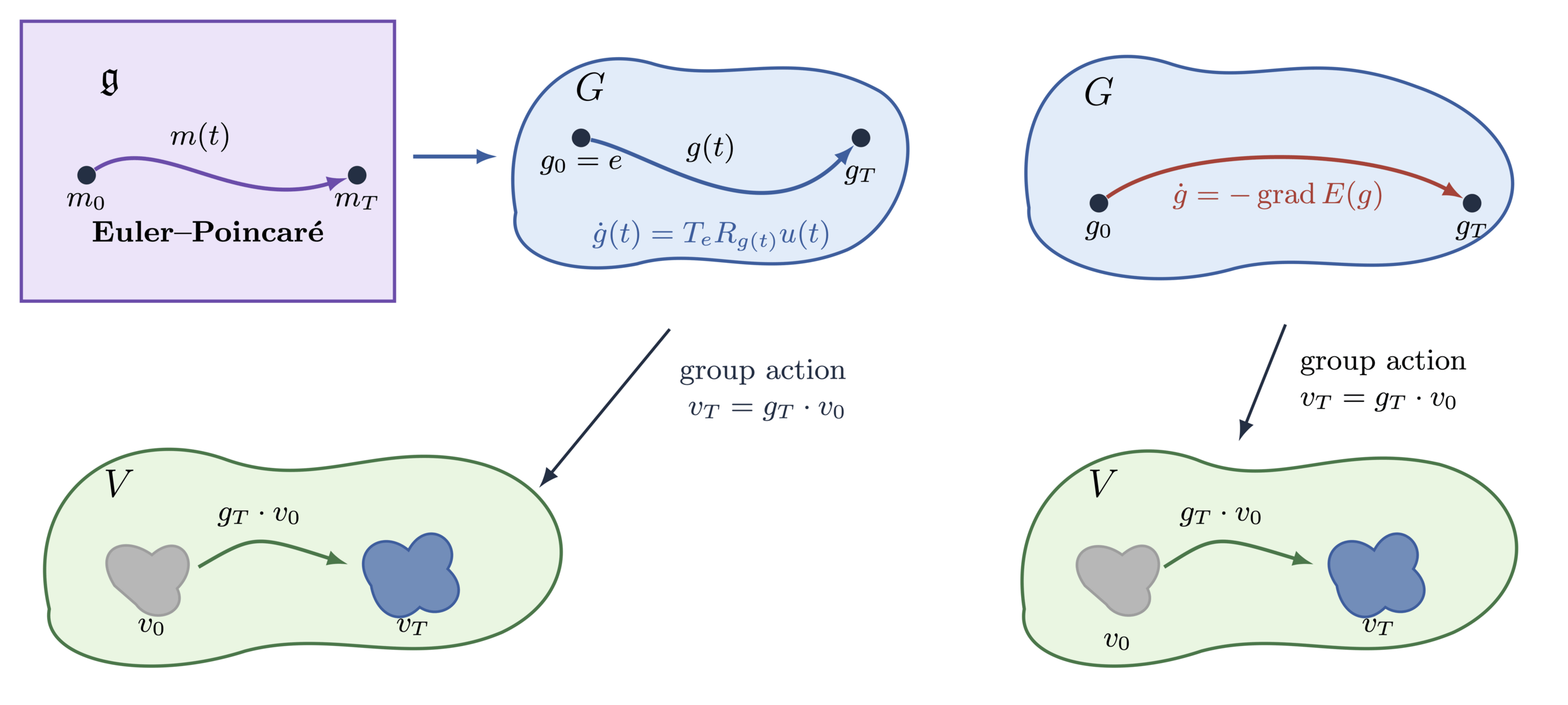
Consider \(\operatorname{Diff}(M)\) as the endpoint of a curve of diffeomorphisms generated by a vector field. Expensive, but geometrically nice (LDDMM!).
By calculus of variations magic, the problem reduces down to solving and analysing a tricky PDE
Issue: Slow, as we need to solve two DEs for each gradient step
Reconstruct the object that gave rise to the data.
Lie Group
of a shape space
acts on an element
\(G\)
\(v\)
\(V\)
\(v\)
Match
in a space
by a forward model
with data
\(d\)
\(Y\)
\(\mathcal{F}\colon V \to Y\)
Example from Lang et al, 2018
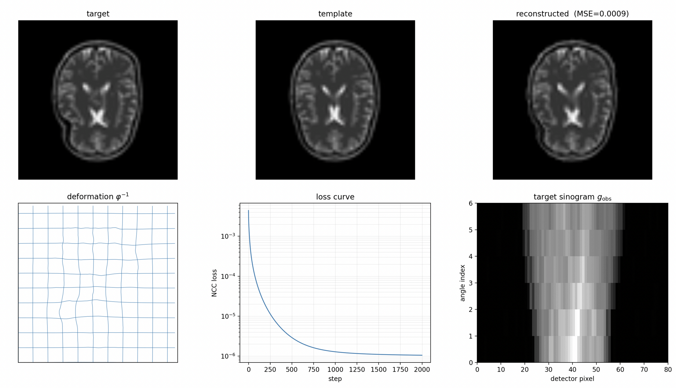
Sinogram (observation)
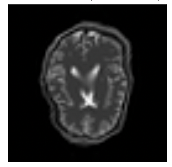
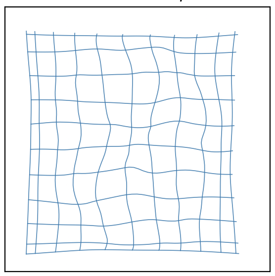
Reconstruction by deformation
Target
Template
Reconstruction by classical methods
Essentially: Solve a variational problem on \(G\), by introducing extra variables,
Iterative updates of infinitesimal generators
One update: solve several DE and compute gradients through these updates
What if we could gradient flow directly on group?
\(\text{iterate}\)
How to compute gradients?
Generally tricky in non-Euclidean setting!
To compute gradients, we need to have a metric.
A clever choice of metric makes the problem tractable.
Translate vectors back to algebra, map one to dual with inertia operator, take duality pairing
The Lie group action on the shape space induces a momentum map
Let \(f\colon V \to \R\) and take \(E(g) = f(\Phi(g,w))\)
\(\Phi\colon G \times V \to V\) is the group action
Why this metric?
Moral of the story: with this choice of metric, the gradient flow has a closed form expression
Ingredients:
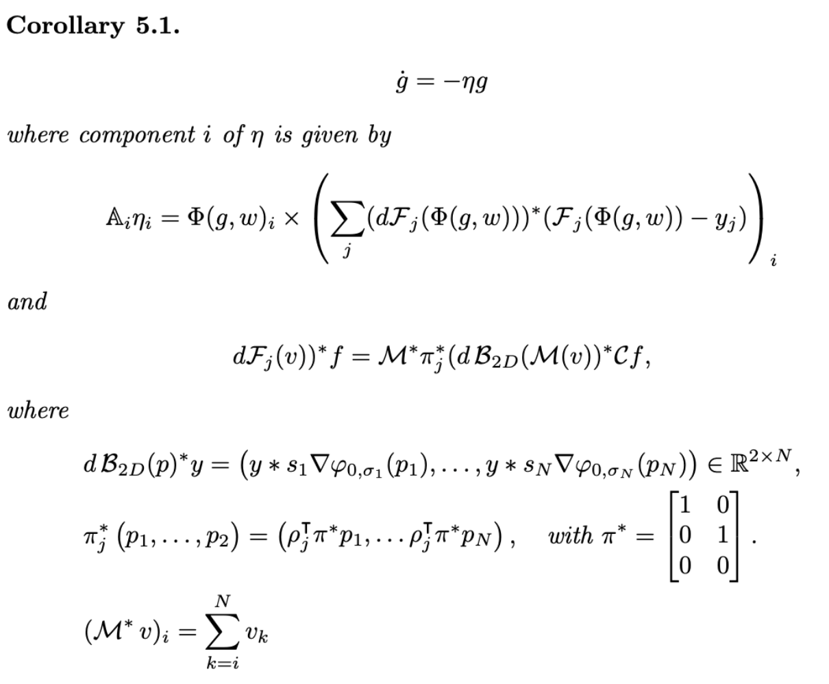
How to construct \(f\)? Take observed data \(y \in Y\) and some data loss \(\mathcal{L}_y \colon Y \to \mathbb{R}\)
Potentially useful
Nice mathematics
Infinite-dimensional geometry
Nonlinear PDE theory
Well-posedness analysis
Geometric mechanics
Nice way of incorporating
anatomical priors
into inverse problems
in 30 seconds (by a maths person)
Electron
microscope
Low dose: low SNR
Many images
Many copies of the same protein but at different orientations and conformations
Particle picking
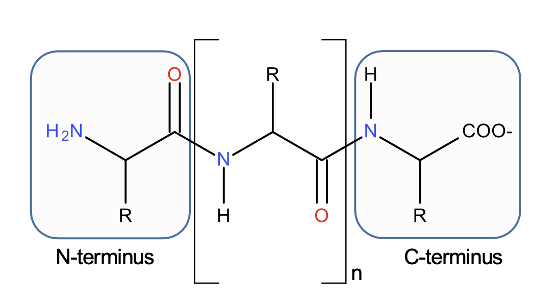
Proteins in 30 seconds (by a mathematician)
In this work: forget about everything but the \(C_\alpha\)s
Relative positions
\((\mathbb R^3)^N\)
Mathematical model for proteins
In the end: Each image with one projection and forward model \(\mathcal{F}_j, j = 1,\ldots, M\)
Shape space: space of relative positions \(V = \mathbb{R}^{3N}\)
Data space - M 2D images, \(L^2(\mathbb{R}^2)^M\)
We want rigid deformations, so \(G = \operatorname{SO}(3)^N\)
\(y_1, \ldots y_M\) are images,
\(\Phi\) is the group action of \(g\)
The adjoint is easy to derive but results in rather unaesthetic expression
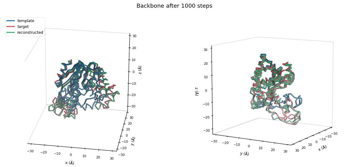
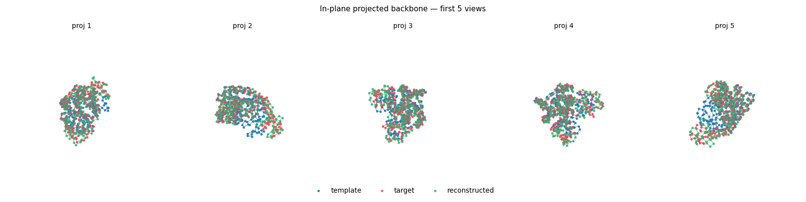
For each image, use NCC similarity, reconstruct by deforming template \(w\)
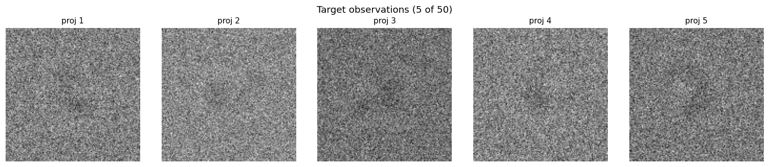
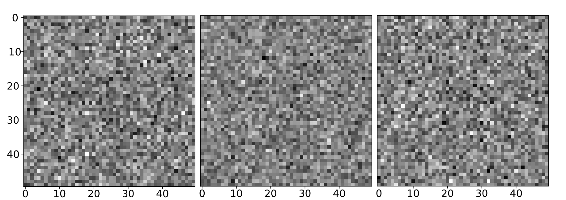
Faint outline of protein can be seen, but \(SNR = 0.01\)
Goal to reconstruct
Template
Find \(g\)
Full protein + 4 Gaussian forward model is used for data generation
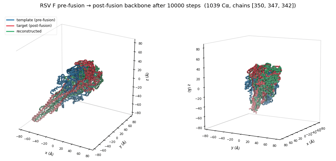
Extension to multi-chain setting is straightforward
Here: 3 Chains, each of ~340 residues, in total 1039 residues
In finite dimensions
(on a compact group)....
Global well-posedness is easy to prove!
As are the properties of the IP
1039 residues is not that much.
Example: EMPIAR-10028 has 80 chains and >10k residues
Template quality?
In this case \(G\) is the set of all diffeomorphisms of the domain, which is inf-dim.
Domain is 2D, so \(\mathbb{R}^2\)
Observations
Ray transform
Angle in [0,60], six angles
Target
in 30 seconds (by a maths person)
X-ray tube
Test object
Detector
Rotation
Momentum map of action \(\Phi(g,w) = w\circ g^{-1}\)
The unregularized gradient flow is given by:
How and why to regularize?
Observations
Reconstruction
Target
Quick!
But now turn up the noise... (a factor 100, so not super realistic)
Reconstruction quality starts to deterioriate!
Framework can handle regularisation as well! But this is a story for another time
Recovers regularization part of a gradient flow from Bauer et al.
Recovers regularization part of a gradient flow from Balehowsky et al.
Extend shape space and re-apply momentum map (which now is a sum)
Big question for me: Well-posedness.
For example, in tomography, pseudodifferential operators inside the GF appears.
Bit messy, but maybe Ebin–Marsden saves the day?
Anatomical priors can be incorporated
using template deformation
Gradient flows speeds up reconstruction
compared to LDDMM-based approaches
A general framework: change problem,
change the ingredients, but geometry
stays the same
By Erik Jansson