































He Wang PRO
Knowledge increases by sharing but not by saving.
王赫
2026/08/09
ICTP-AP, UCAS
hewang@ucas.ac.cn
PART 3: Transformer + LLM + Agent + Harness
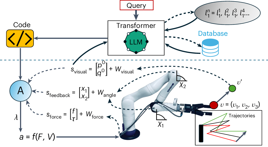
接下来开始新的最后章节,主要是涉及从2025到2026年以来Harness 的内容。将会涉及到“测试语言模型作为AI Agent 的能力”(借鉴李宏毅的案例来说明Agent的Harness底层是是如何工作的);分清楚AI Agent=LLM+Harness;Vibe Coding vs Context Engineering vs Harness Engineering;控制认知框架 AGENTS.md, CLAUDE.md;控制能力边界 SWE-agent;用标准工作流程来控制“行为”https://ghuntley.com/ralph/
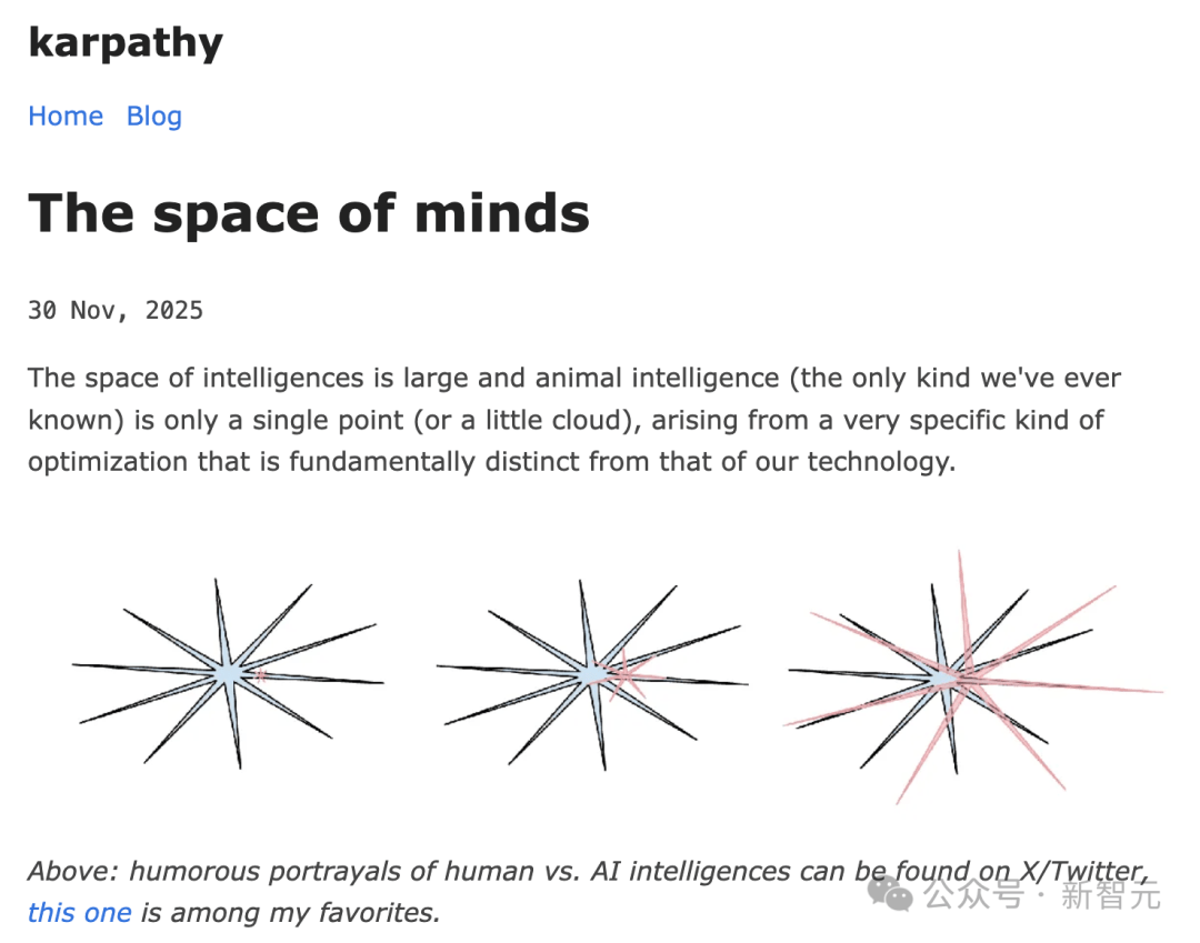
https://ghuntley.com/loop/ https://arxiv.org/pdf/2603.26177v1 ; 过度责备AI Agent可能有害;Life-long AI Agent Harness 之 自动更新模型参数 https://arxiv.org/pdf/2603.12273 ;Life-long AI Agent Harness 之自动更新harness https://arxiv.org/abs/2603.28052 ;国内中转站; 那些Harness当红辣子鸡:Codex vs Claude Code vs ... ;我们日常应该如何能更大限度发挥 AI Agent的能力呢?(强且合适的LLM(Karpathy关于Space of Minds的图) + 善用Harness(展示流形空间上可以如何提问或者被问来获取新知))
What Is Machine Learning?
— The basics and why it mattersDeep Learning: When Machines Start to See and Think
— From neural networks to powerful representations
Gravitational Waves Meet Machine Learning
— How ML is reshaping data analysis in GW astronomy
Let’s Get Practical: Searching for Gravitational Waves
— A hands-on look at applying ML in real GW searches
LLMs for Gravitational Waves: My Ongoing Work
— Towards automated and interpretable scientific discovery
Natural Language Processing (NLP) = teaching computers to work with human language
# NLP
Human language → something computers can recognize, understand, predict, and generate
Before LLMs: one task, one model.
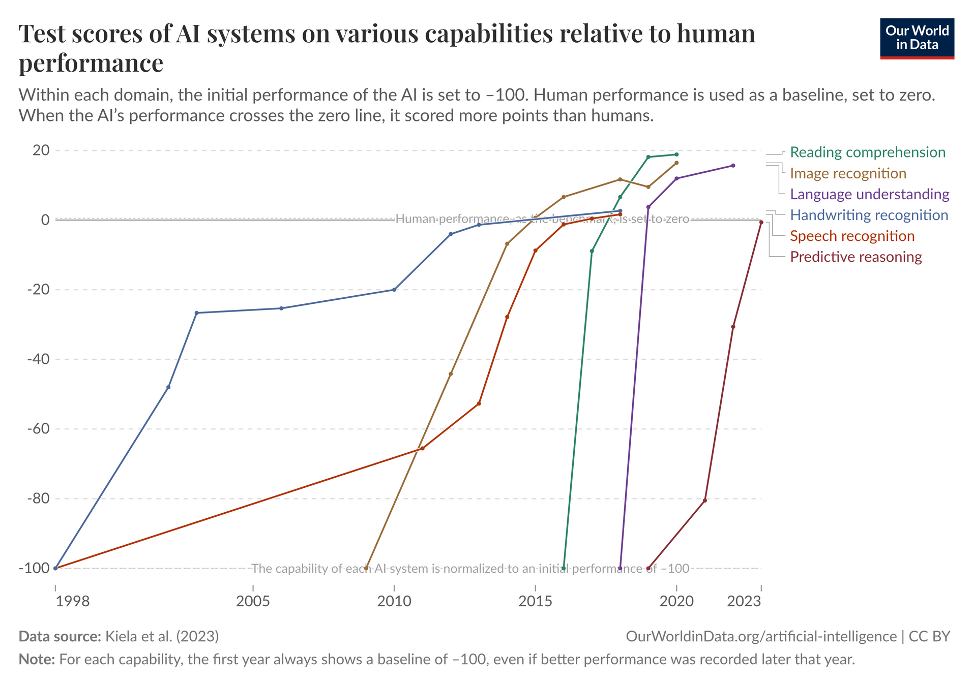
AI capabilities were improving — but separately.
Before LLMs: one task, one model.
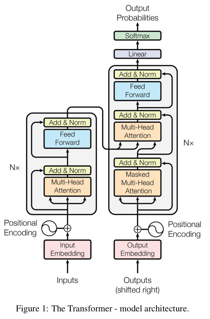
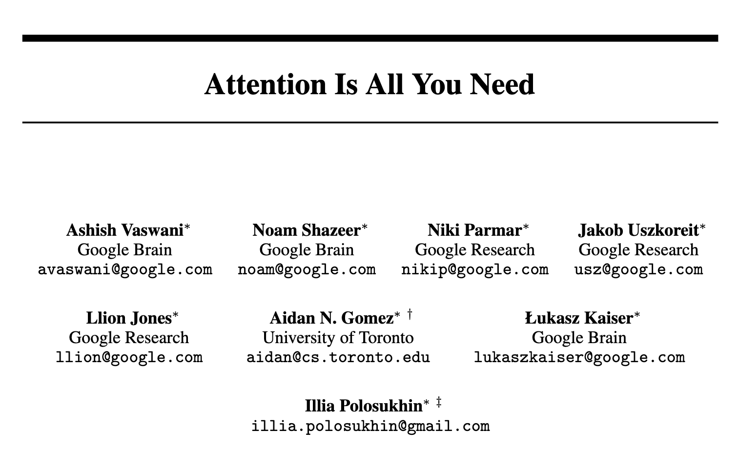
“Attention Is All You Need” — from recurrent processing to attention-based sequence modeling
# NLP
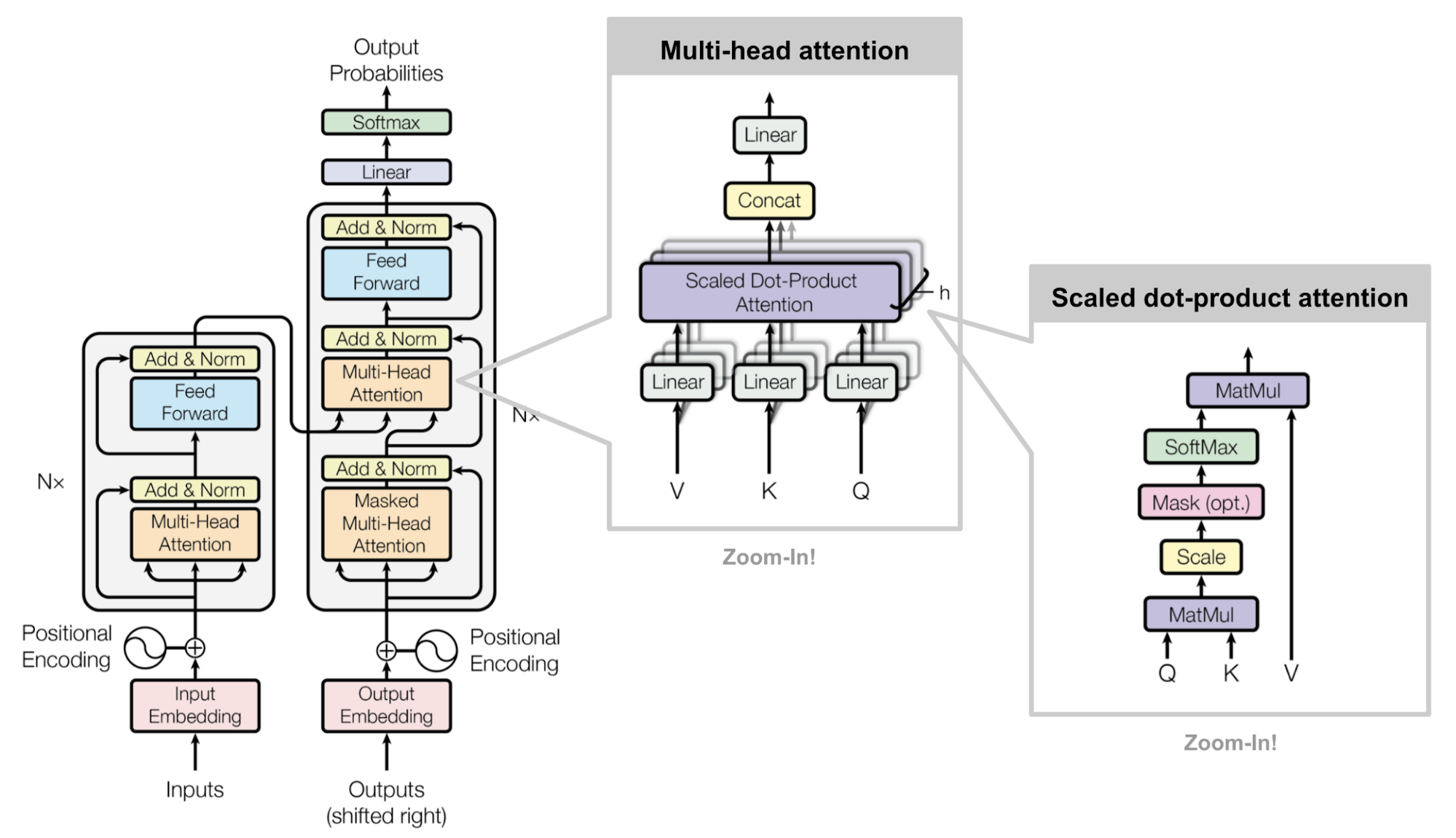
The original Transformer was built for machine translation, not for ChatGPT.
A paper for machine translation became the foundation of modern LLMs.
This architecture will be our map for the next few slides.
arXiv:1706.03762 [cs.CL]
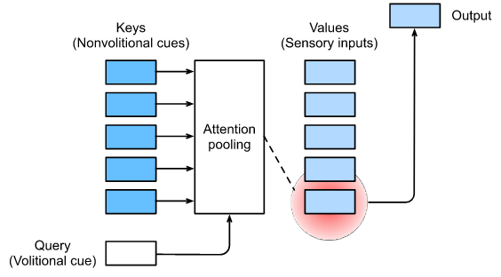
Attention: “What should I look at?”
# NLP
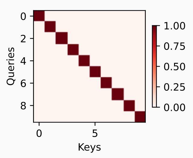
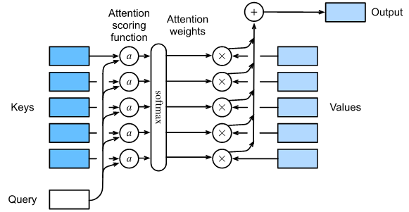
Given a query, attention measures its relevance to all keys, then uses these scores to combine the corresponding values.
Query
Key
Value
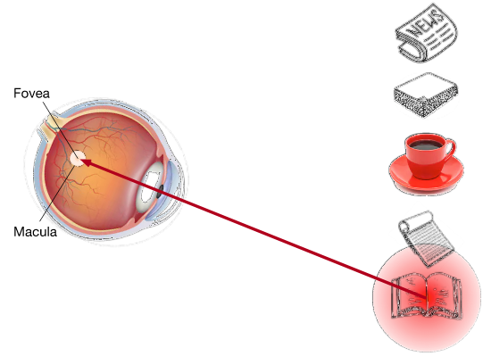
We do not process everything equally.
We focus on what is relevant.
Human intuition
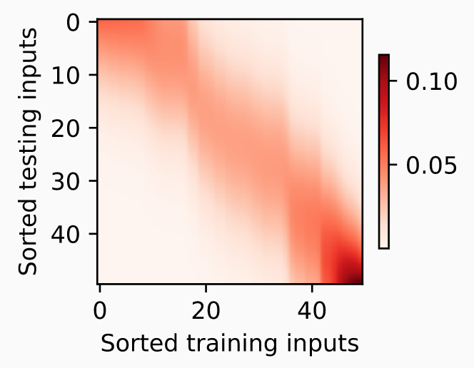
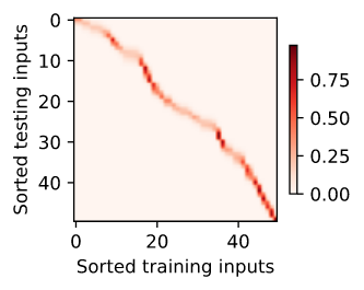
Attention Heatmap
(Color = attention weight)
Attention = Learn How Much Each Example Matters
# NLP
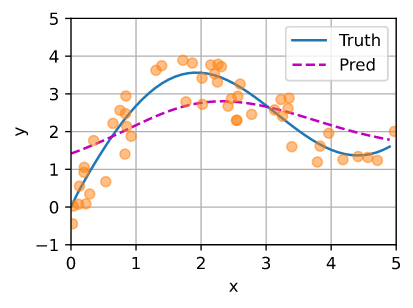
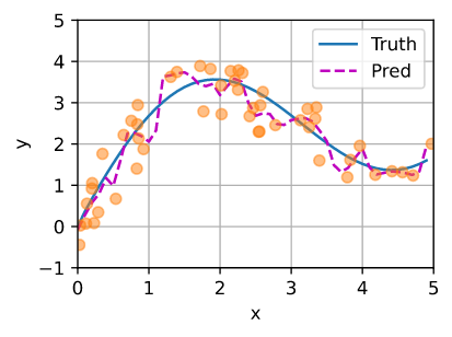
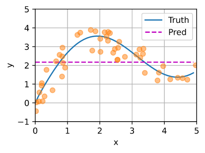
Consider a simple regression problem:
The key question is: should every training point contribute equally?
Case 1: Average Pooling
Case 2: Nonparametric Attention Pooling
Case 3: Parametric Attention Pooling
Everyone matters equally
Ignores the query x.
Data:
\(\omega\) controls how selective the attention is — and it can be learned from data.
Attention Scoring Functions
# NLP
Query–Key similarity determines how much Value information is retrieved.
给定一个 query q 和一组 key–value pairs \((k_i,v_i)\),
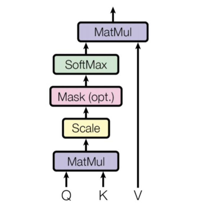
Transformer chooses a simple scoring function: dot product
queries \(Q \in \mathbb{R}^{n \times d}\), keys \(K \in \mathbb{R}^{m \times d}\) 和 values \(V \in \mathbb{R}^{m \times v}\) :
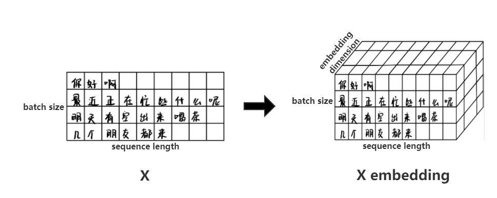
Q/K/V ~ [batch_size,len_tokens,dim_features]
[b, 15, 10]
[b, 15, 13]
[b, 15, 11]
[b, 13, 10]
[b, 13, 11]
In high dimensions, dot products become large; scaling keeps softmax from becoming too saturated.
Multi-Head Attention & Self-Attention
# NLP
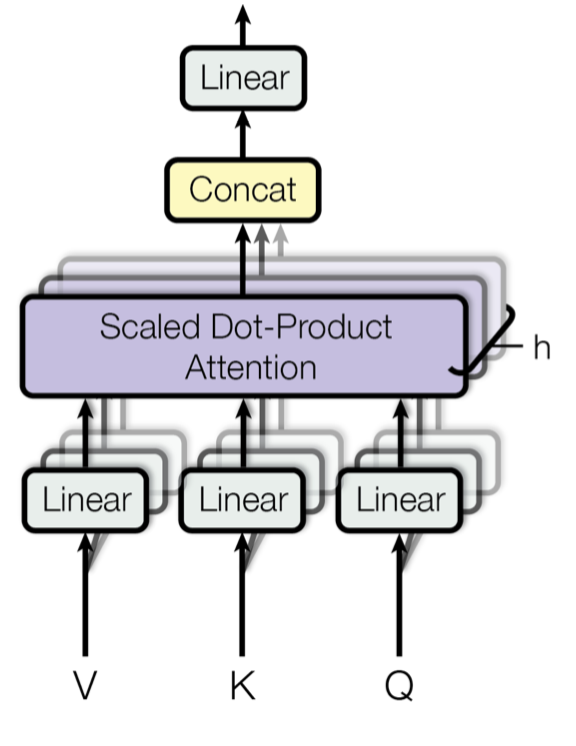
单个 attention 只在一个表示空间里衡量相关性;Multi-Head Attention 让模型同时从多个表示子空间观察同一组 token。
Note: More heads ≠ simply more copies of the same attention. Each head has its own learned projections \(W_i^Q,W_i^K,W_i^V\).
Self-attention means Q, K, and V are all derived from the same input sequence X. Each token looks at other tokens in the same sequence.
[batch_size * num_heads,
len_tokens,
dim_features / num_heads]
Q,K,V ~ [batch_size, len_tokens, dim_features]
[batch_size,
 len_tokens,
 dim_features]
[b, 5, 10]
[b, 5, 10]
[bx2, 5, 5]
(h=2)
Positional Encoding: Attention Has No Sense of Order
# NLP
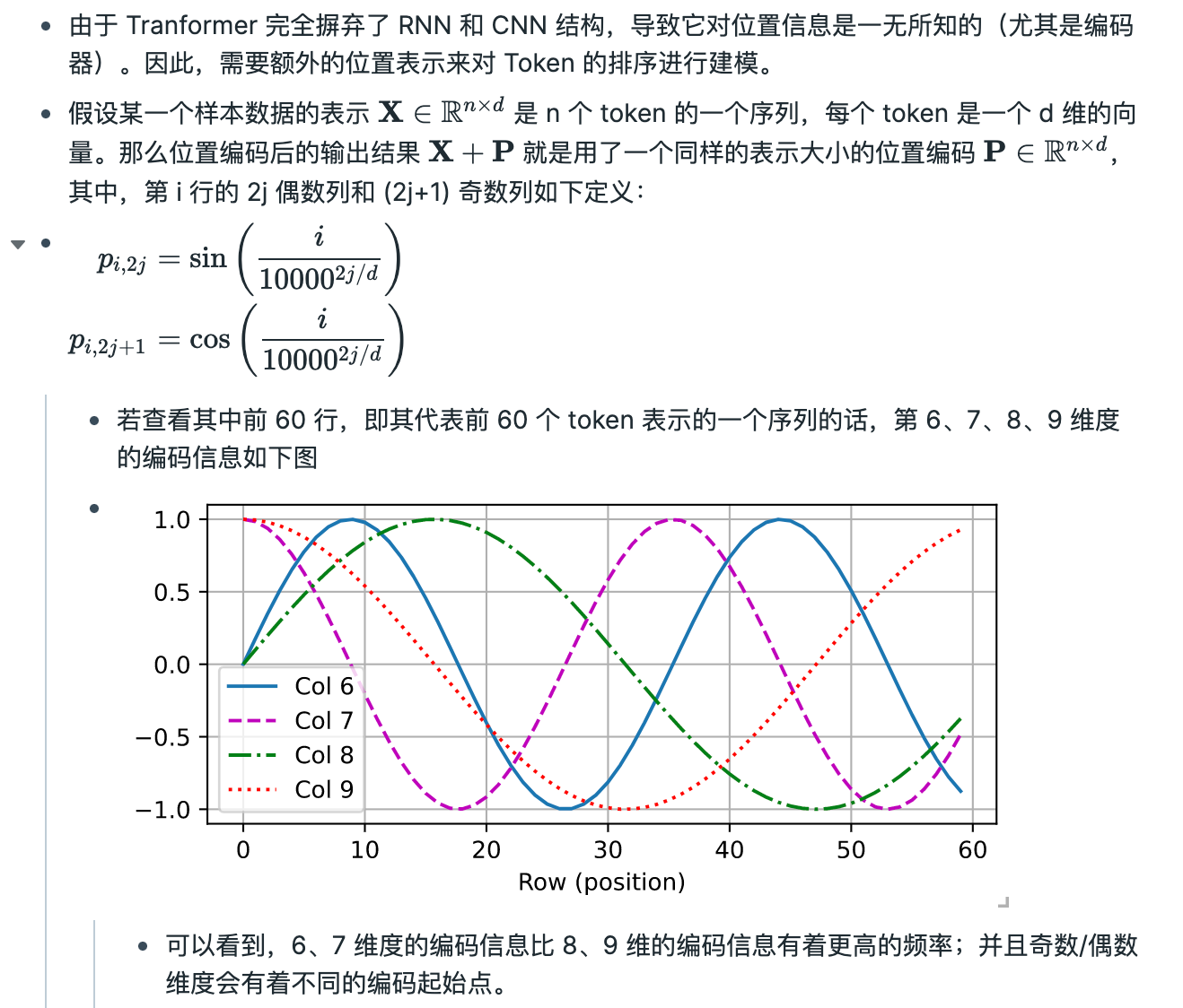
Self-attention itself is permutation-insensitive: without extra position information, it does not know the order of tokens.
[batch_size, len_tokens]
[batch_size,
 len_tokens,
 dim_features]
[batch_size,
 len_tokens,
 dim_features]
Token embedding
“What is this token?”
Positional encoding
“Where is this token?”
这意味着模型不仅能知道“token 在第几个位置”,还比较容易从表示中学习“两个 token 相隔多远”。
Modern LLMs often use other schemes, e.g. learned embeddings or RoPE.
Feed-Forward + Add & Norm
# NLP
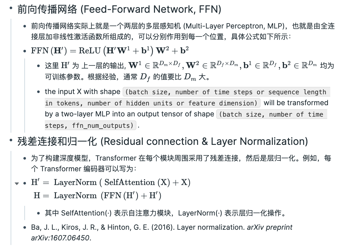
Attention mixes tokens; FFN transforms each token.
[batch_size,
 len_tokens,
 dim_features]
[batch_size,
 len_tokens,
 dim_features]
[batch_size, len_tokens, dim_features]
K
V
Q
# NLP
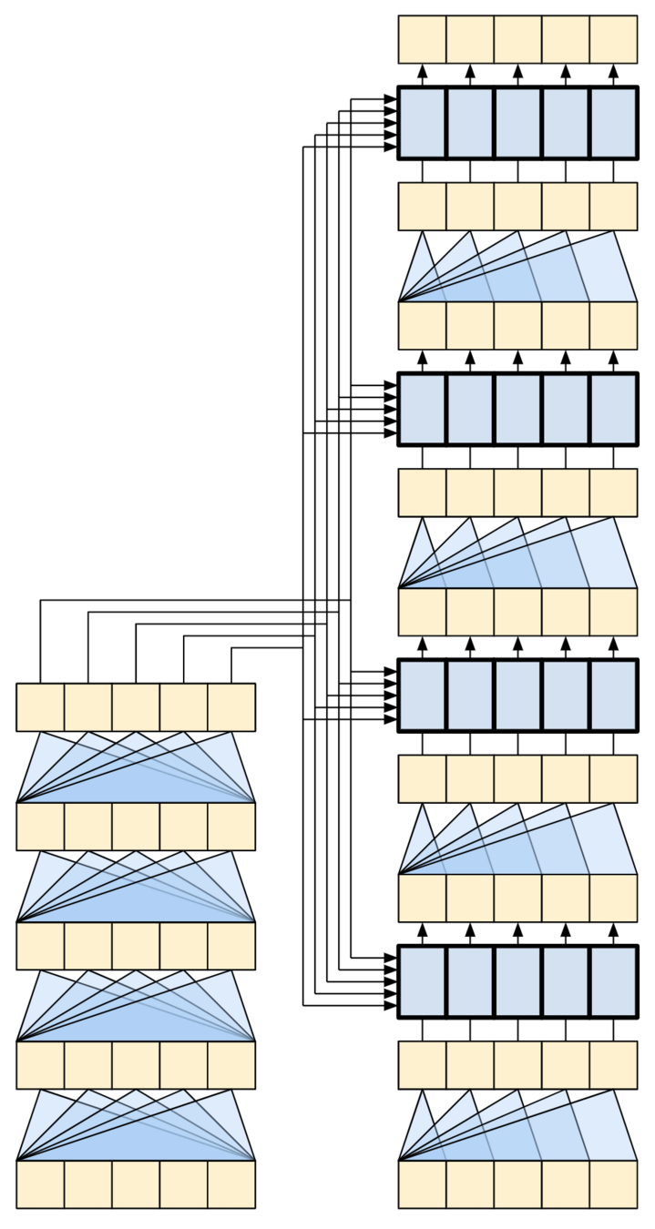
Now we can read the whole Transformer from bottom to top.
Q from Decoder
K,V from Encoder
[batch_size,
 len_tokens1,
 dim_features1]
[batch_size, len_tokens2]
[batch_size, len_tokens2, vocal_size]
K
V
Q
[batch_size,
 len_tokens1,
 dim_features1]
[batch_size,
 len_tokens2,
 dim_features2]
[batch_size, len_tokens1]
, len_tokens1]
# NLP
[batch_size,
 len_tokens1,
 dim_features1]
[batch_size, len_tokens1]
[batch_siz
[batch_size, len_tokens2, vocal_size]
[batch_size,
 len_tokens1,
 dim_features1]
[batch_size,
 len_tokens2,
 dim_features2]
K
V
Q
Now we can read the whole Transformer from bottom to top.
[batch_size, len_tokens2]
, len_tokens1]
Source: X
# NLP
[batch_size,
 len_tokens1,
 dim_features1]
[batch_size, len_tokens1]
[batch_siz
[batch_size, len_tokens2, vocal_size]
[batch_size,
 len_tokens1,
 dim_features1]
[batch_size,
 len_tokens2,
 dim_features2]
K
V
Q
Now we can read the whole Transformer from bottom to top.
[batch_size, len_tokens2]
, len_tokens1]
Source: X
Source: X
# NLP
[batch_size, len_tokens2, vocal_size]
Source: X
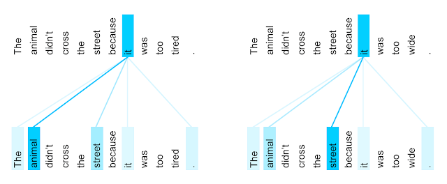
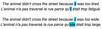
The encoder self-attention distribution for the word “it” from the 5th to the 6th layer of a Transformer trained on English to French translation (one of eight attention heads).
What Does Self-Attention Learn?
Same word, different context → different reference
Query: “it”
Keys: all words in the sentence
Attention weight: how strongly “it” attends to each word
One step to connect distant tokens — and we can visualize the connection.
# NLP
["This", "is", "a", "sample"]
[1, 16512]
[1, 128, 256]
HW+ , MLST (2024)
# NLP
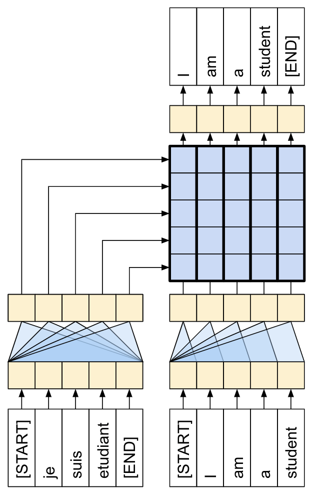
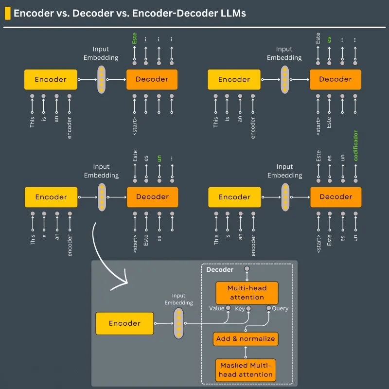
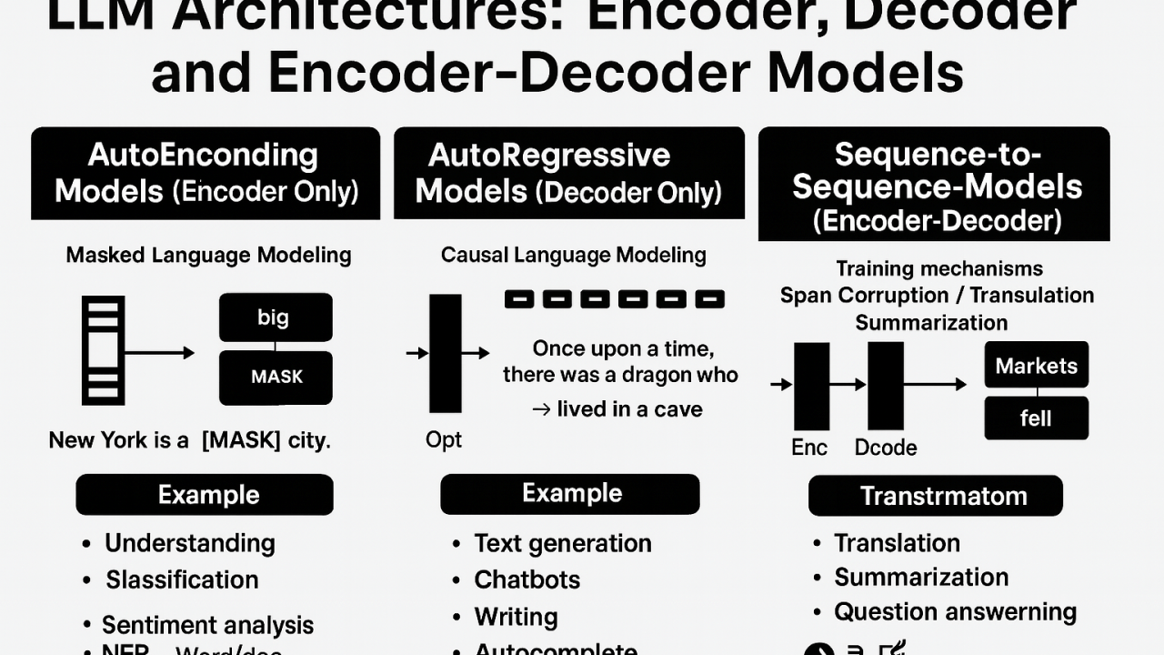
Encoder vs. Encoder–Decoder vs. Decoder
Source: X
Read everything
典型任务:classification · retrieval · NER · embeddings
Read, then generate
Predict what comes next
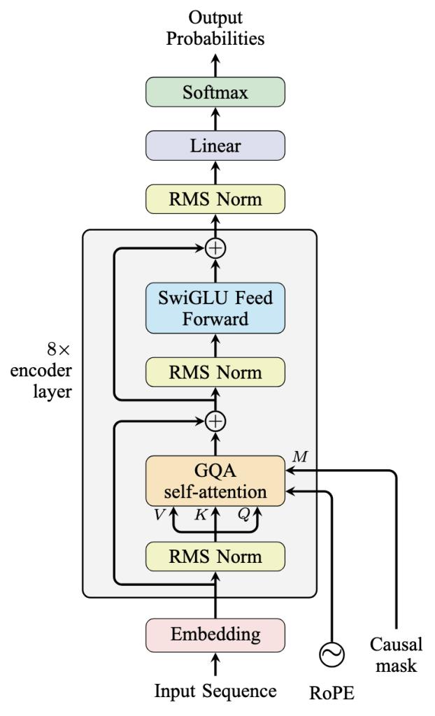
Decoder-Only Model Following the Architecture of Llama-2/Llama-3
Source: X
# NLP
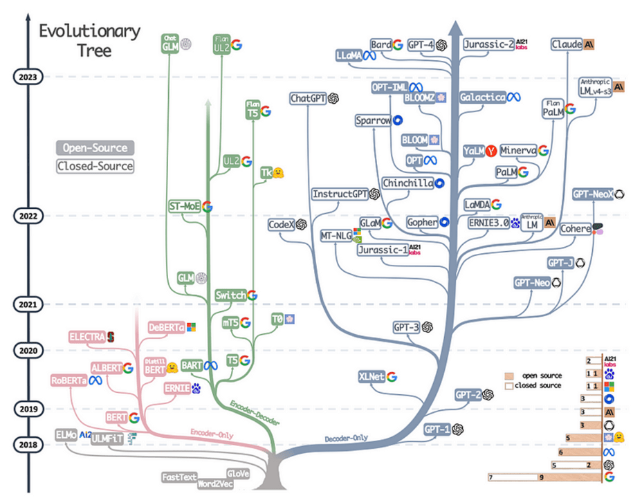
Three branches emerged — but one became dominant for general-purpose LLMs.
\(\text{The cat sat on the} \rightarrow ?\)
Predict next token.
Causal
Generation-oriented
\(\text{The cat [MASK] on the mat}\)
Predict masked token.
Bidirectional
Representation-oriented
Excellent representations / understanding
The path that scaled into general-purpose LLMs
BERT looked extremely powerful
GPT-style scaling changed the game
GPT-style scaling changed the game
Excellent sequence-to-sequence models
# LLM
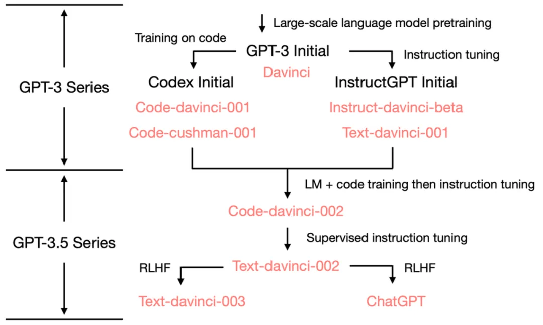
Training on code did more than teach the model programming.
GPT-3 (2020)
ChatGPT (2022)
Magic: Code + Text
John has 3 apples and buys 2 more.
How many does he have?
apples = 3
apples += 2
print(apples)Natural language
Code
Training on code did more than teach the model programming.
GPT-3 (2020)
ChatGPT (2022)
Magic: Code + Text
John has 3 apples and buys 2 more.
How many does he have?
apples = 3
apples += 2
print(apples)Natural language
Code
# LLM
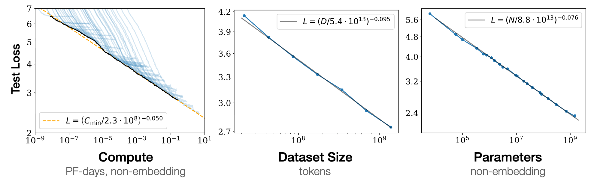
More compute, more data, larger models → predictably lower loss
Predictable
Continuous
Composable
arXiv:2001.08361 [cs.LG]
Performance did not saturate as quickly as people expected.
# LLM
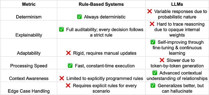
From explicit rules to natural-language control
Rule-Based Vs. LLMs: (Source)
if sender in VIP_LIST \
   or "urgent" in subject \
   or "!" in subject \
   or priority == "high":
    notify()
❌ brittle rules
❌ unseen wording
❌ endless edge cases
Program the condition
Describe the condition
if LLM(
  "Does this message require
   an important action soon?"
):
    notify()
如果收到一封“重要且需要我尽快处理”的邮件,就提醒我。
✓ semantic
✓ context-aware
✓ adaptable to unseen cases
# LLM
From explicit rules to natural-language control
Rule-Based Vs. LLMs: (Source)
# LLM
From explicit rules to natural-language control
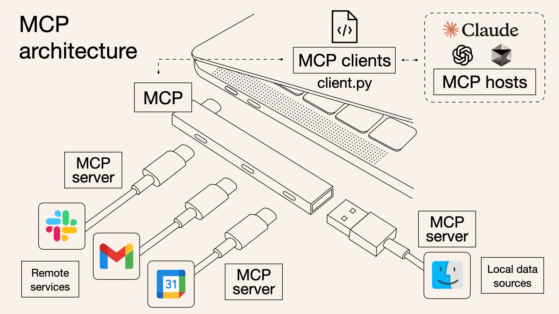
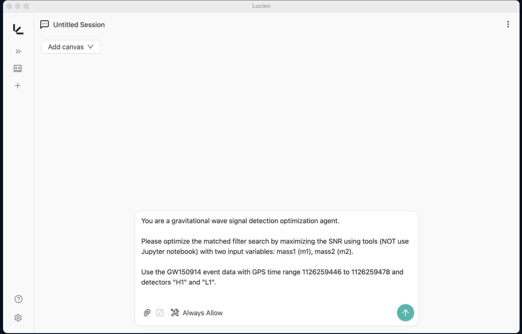
模型上下文协议(Model Context Protocol,MCP),是由Anthropic推出的开源协议,旨在实现大语言模型与外部数据源和工具的集成,用来在大模型和数据源之间建立安全双向的连接。
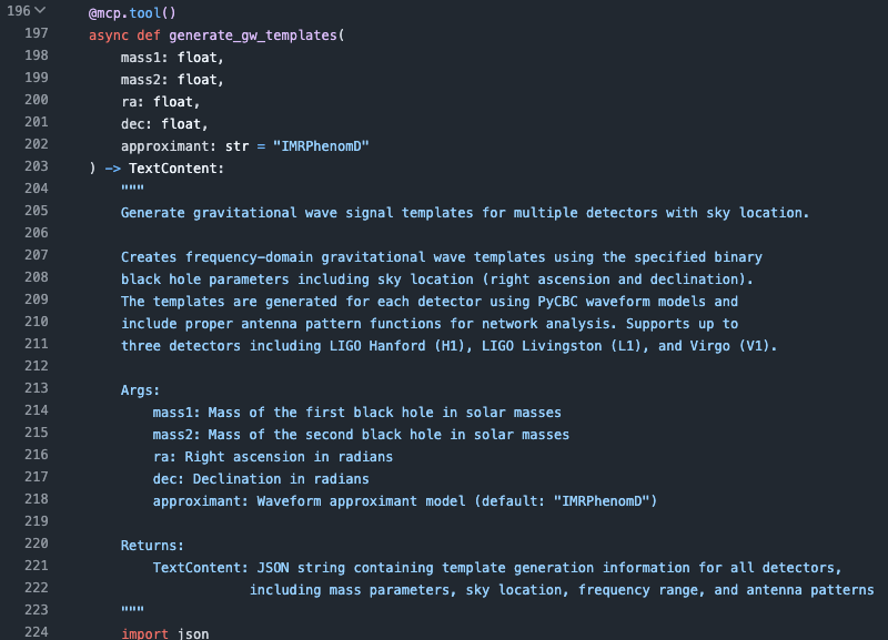
MCP Tool
prompt
"Please generate gw templates first."Demo: GW150914 MCP Signal Search
# LLM
From explicit rules to natural-language control
if chi_square > 10:
rerun_analysis()Program the condition
Describe the condition
if LLM(
    """
    Given the diagnostic plots, residuals,
    logs, and previous runs:
    does this result show evidence of
    a meaningful model-data mismatch
    that warrants another analysis?
    """
):
    rerun_analysis()
以前
condition必须是一个程序员提前定义好的数值判据。
现在 condition 可以是对文本、图像、日志、上下文甚至科研语义的综合判断。
# LLM
# Agent
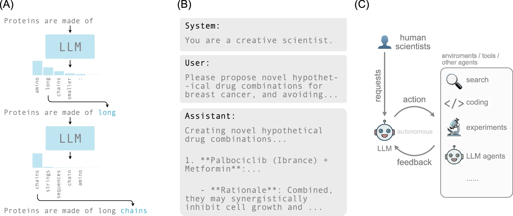
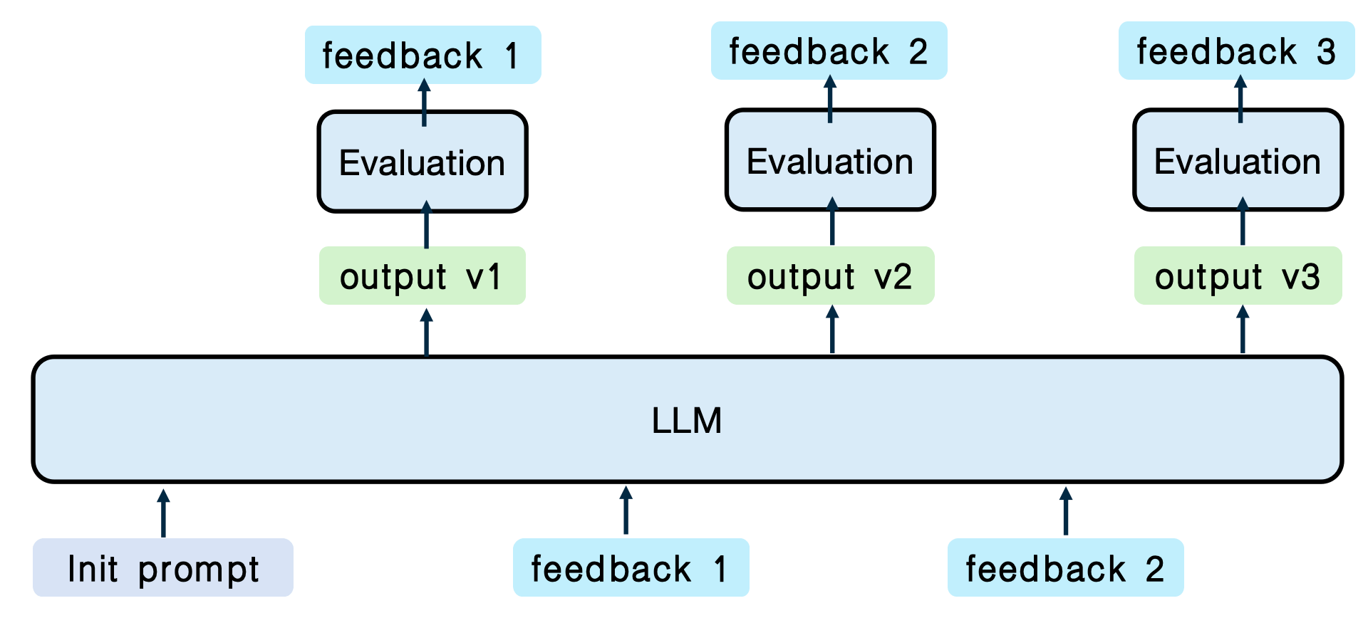
Generate → Observe → Act → Refine
One-shot generation → iterative interaction
直接不行?那就包装回炉再来一遍。
npj Artif. Intell. 1, 14 (2025).
"序列生成"
"序列输入"
"Direct fails. Refine and recover."
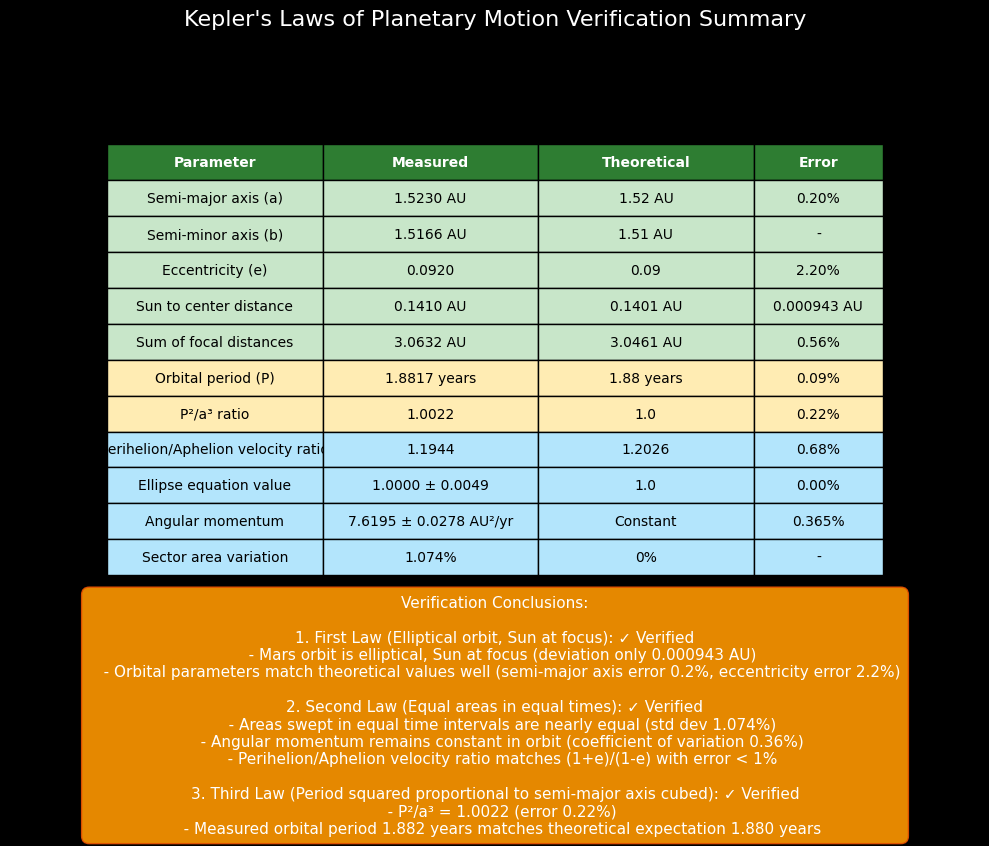
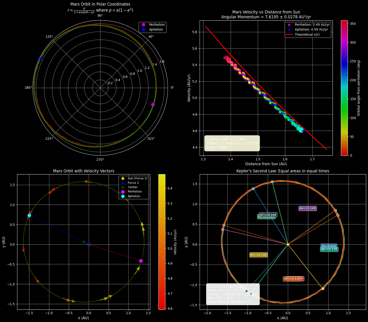
Demo: LLM 验证开普勒行星运动三定律
# Agent
Agent 并不一定意味着我们发明了一个全新的模型。
很多时候,它只是把 LLM 放进了一个“观察—决策—行动—反馈”的循环里。
One-shot generation → iterative interaction
直接不行?那就包装回炉再来一遍。
npj Artif. Intell. 1, 14 (2025).
"序列生成"
"序列输入"
"Direct fails. Refine and recover."
Generate → Observe → Act → Refine
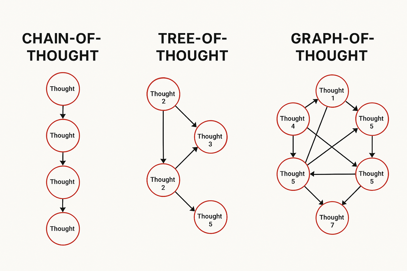
arXiv:2201.11903 [cs.CL]
arXiv:2305.10601 [cs.CL]
# Agent
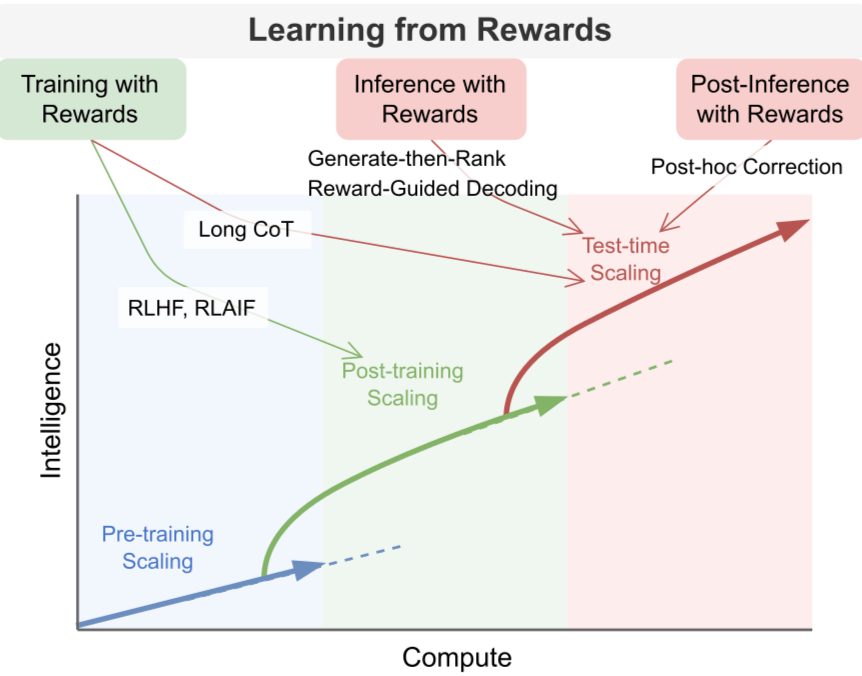
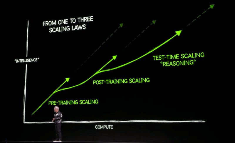
Pre-training scaling
\(\text{more parameters + data + compute}\)
→ build a stronger base model
↓
Post-training scaling
\(\text{more post-training data + optimization / RL compute}\)
→ teach better behavior and reasoning
SFT · RLHF/RLAIF · RL for reasoning
↓
Test-time scaling
\(\text{more inference compute per problem}\)
→ spend more compute on one problem
longer reasoning · multiple samples · search · verification
More compute, at different stages
📄 Google DeepMind: "Scaling LLM Test-Time Compute Optimally" (arXiv:2408.03314)
🔗 OpenAI: Learning to Reason with LLMs
# Agent
Pre-training scaling
\(\text{more parameters + data + compute}\)
→ build a stronger base model
↓
Post-training scaling
\(\text{more post-training data + optimization / RL compute}\)
→ teach better behavior and reasoning
SFT · RLHF/RLAIF · RL for reasoning
↓
Test-time scaling
\(\text{more inference compute per problem}\)
→ spend more compute on one problem
longer reasoning · multiple samples · search · verification
More compute, at different stages
# Agent
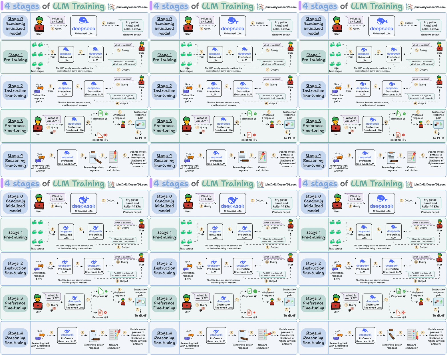
Pre-train → Instruct → Align → Reason
Source: X
# Agent
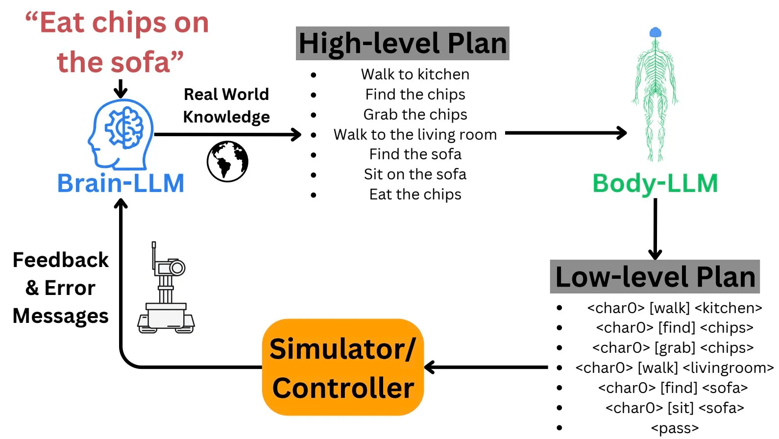
Put an LLM inside a world — and let it remember, plan, and act
Generative behavior emerges inside a carefully engineered rule scaffold. 🤫
arXiv:2304.03442 [cs.HC]
Source: X
Search, Optimization, and Automated Scientific Reasoning
# Agent
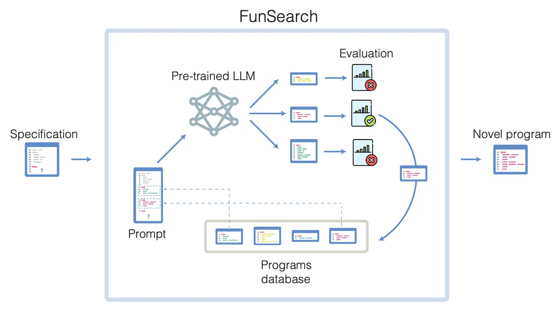
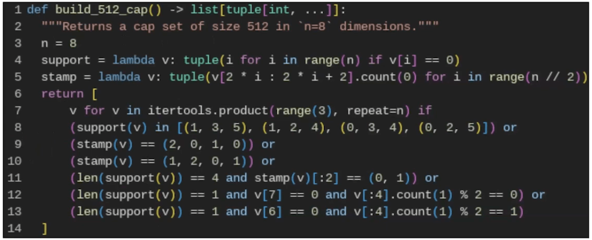
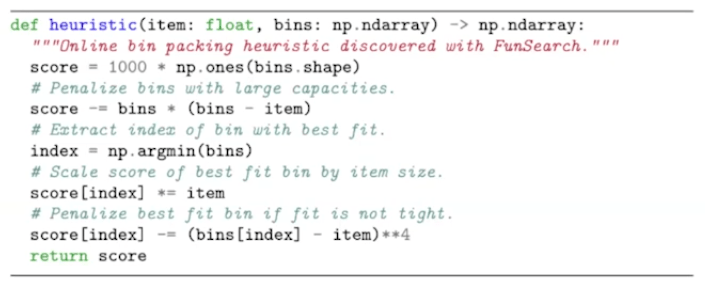
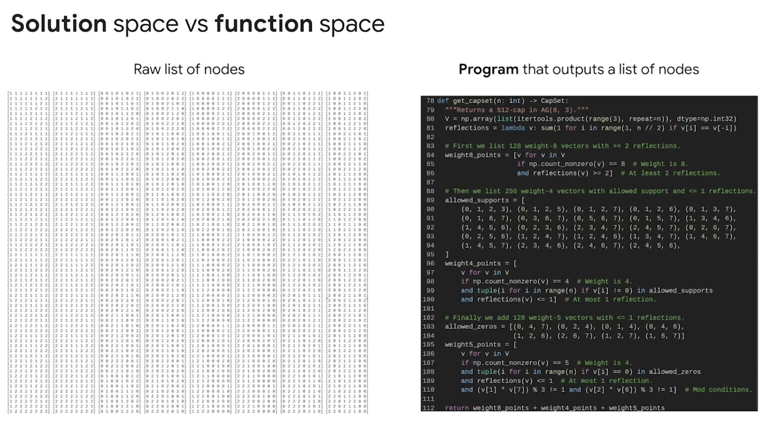
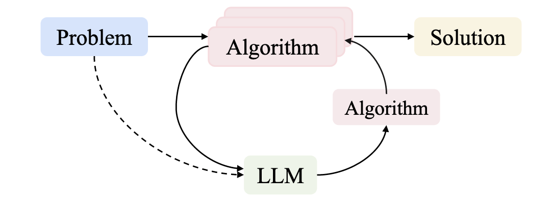
Search for programs that solve the problem, not for the solution itself.
Illustrative example of bin packing using existing heuristic – Best-fit heuristic (left), and using a heuristic discovered by FunSearch (right).
DeepMind Blog (Source)
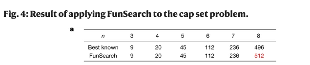
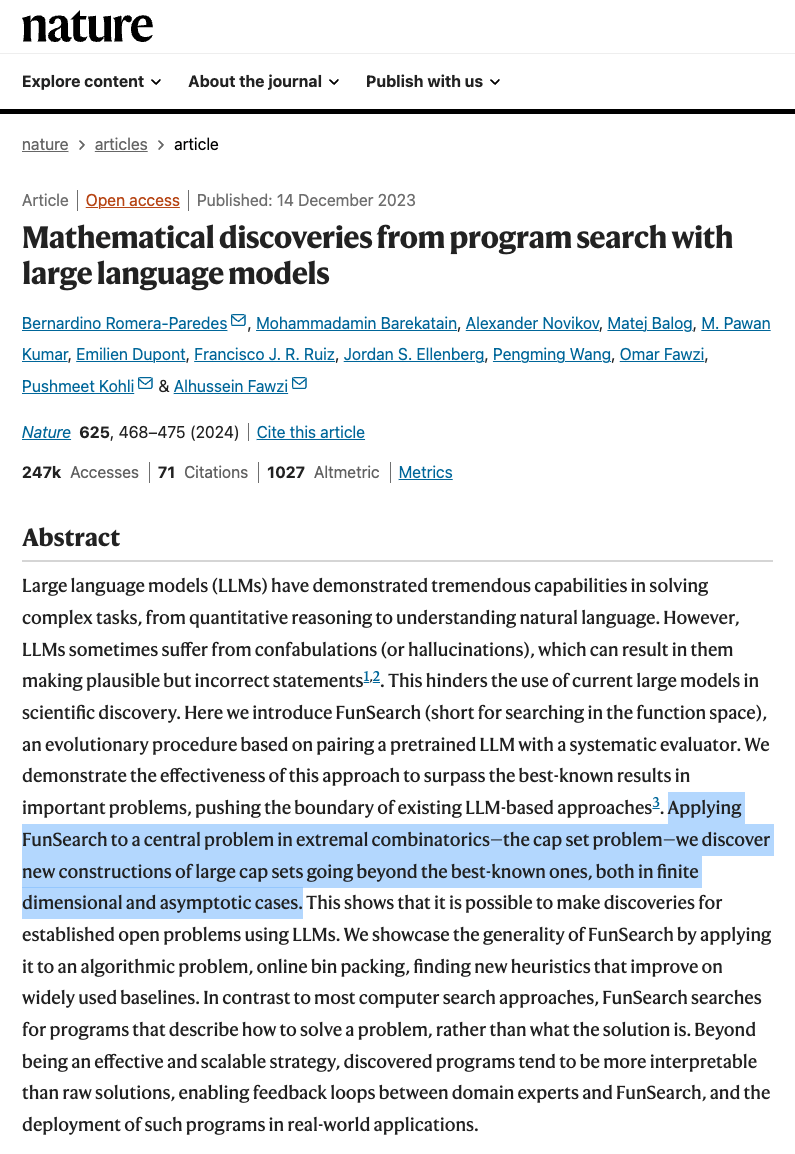
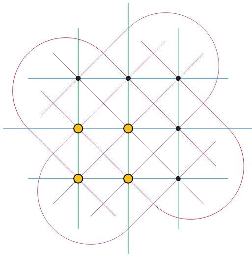
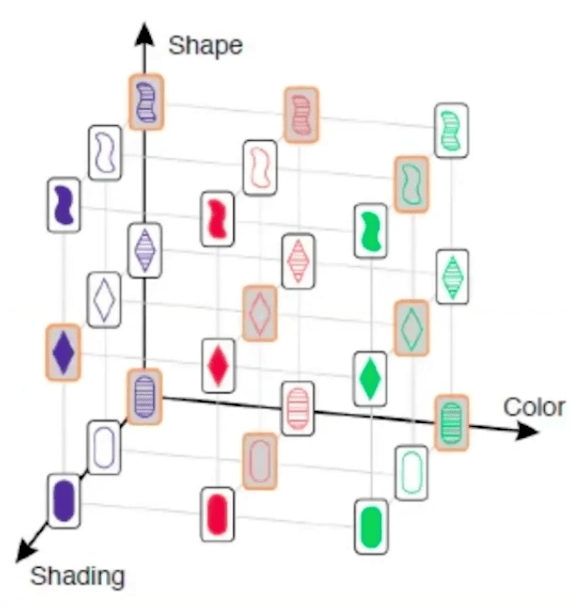
Cap Set Problem
Bin Packing Problem
The largets cap set in N=2 has size 4.
The largest cap set in N=3 has size 9 > \(2^3\)
For N > 6, the size of the largest cap set is unknown.
# Agent
Search for programs that solve the problem, not for the solution itself.
Real-world Case: FunSearch (Nature, 2023)
YouTube (Source)
Generate → Execute → Score → Select → Generate again
# Agent
Why Search in Program Space?
YouTube (Source)
# Agent
From solving instances to searching for reusable algorithms
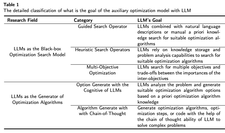
Two Directions of LLM-based Optimization
arXiv: 2405.10098 [cs.LG]
arXiv:2410.14716 [cs.LG]
Direction 2 — LLM as algorithm designer
Search for a heuristic / program / solver
\(\text{problem class}\rightarrow\text{LLM + search}\rightarrow\text{algorithm}\rightarrow\text{many instances}\)
Much more interesting for scientific discovery.
# Agent
The bottleneck is no longer generating algorithms — it is how to explore the algorithm space.
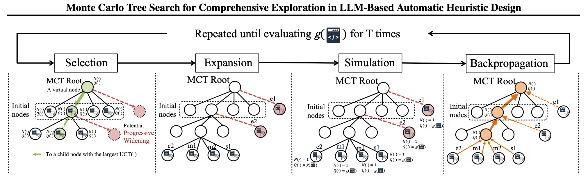
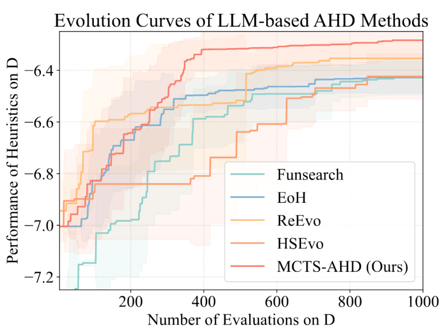
MCTS-AHD
arXiv:2501.08603 [cs.AI]
Good branches receive more search budget, while unexplored branches are still sampled.
Search organization matters.
arXiv:2402.01145 [cs.NE]
ReEvo
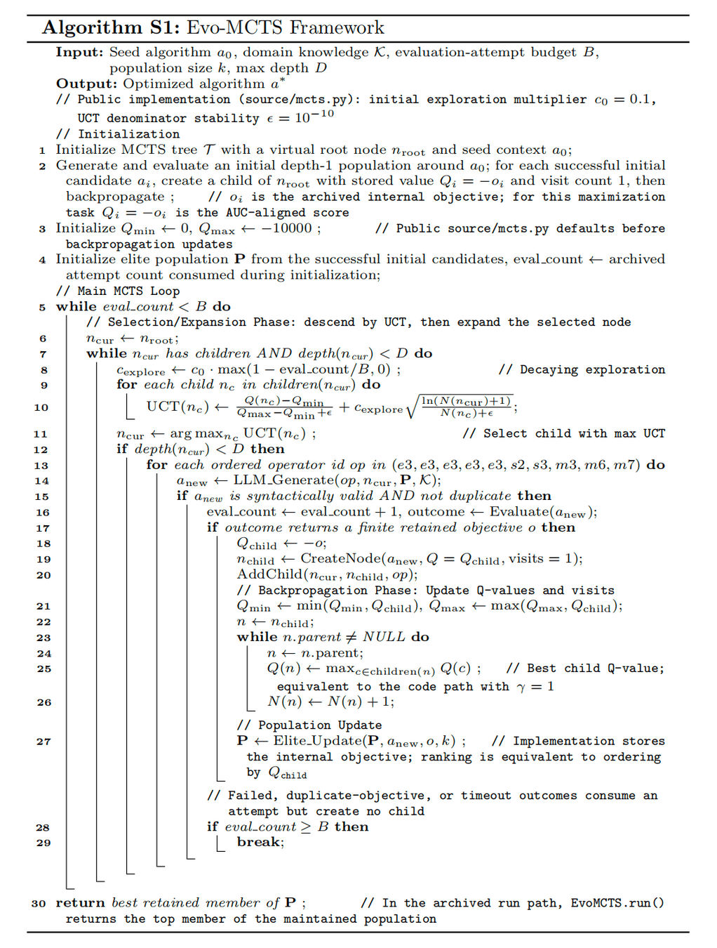
# Evo-MCTS
The target is not another black-box model — but interpretable, executable analysis logic.
Motivation I — Hand-designed model-based pipelines
Motivation II — Black-box data-driven pipelines
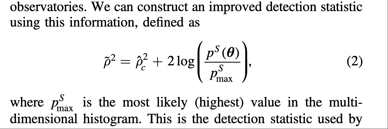
Nitz et al., ApJ (2017)
Sci4MLGW@ICERM (June 2025)
A precedent: improving a classical statistic using learned / empirical prior information
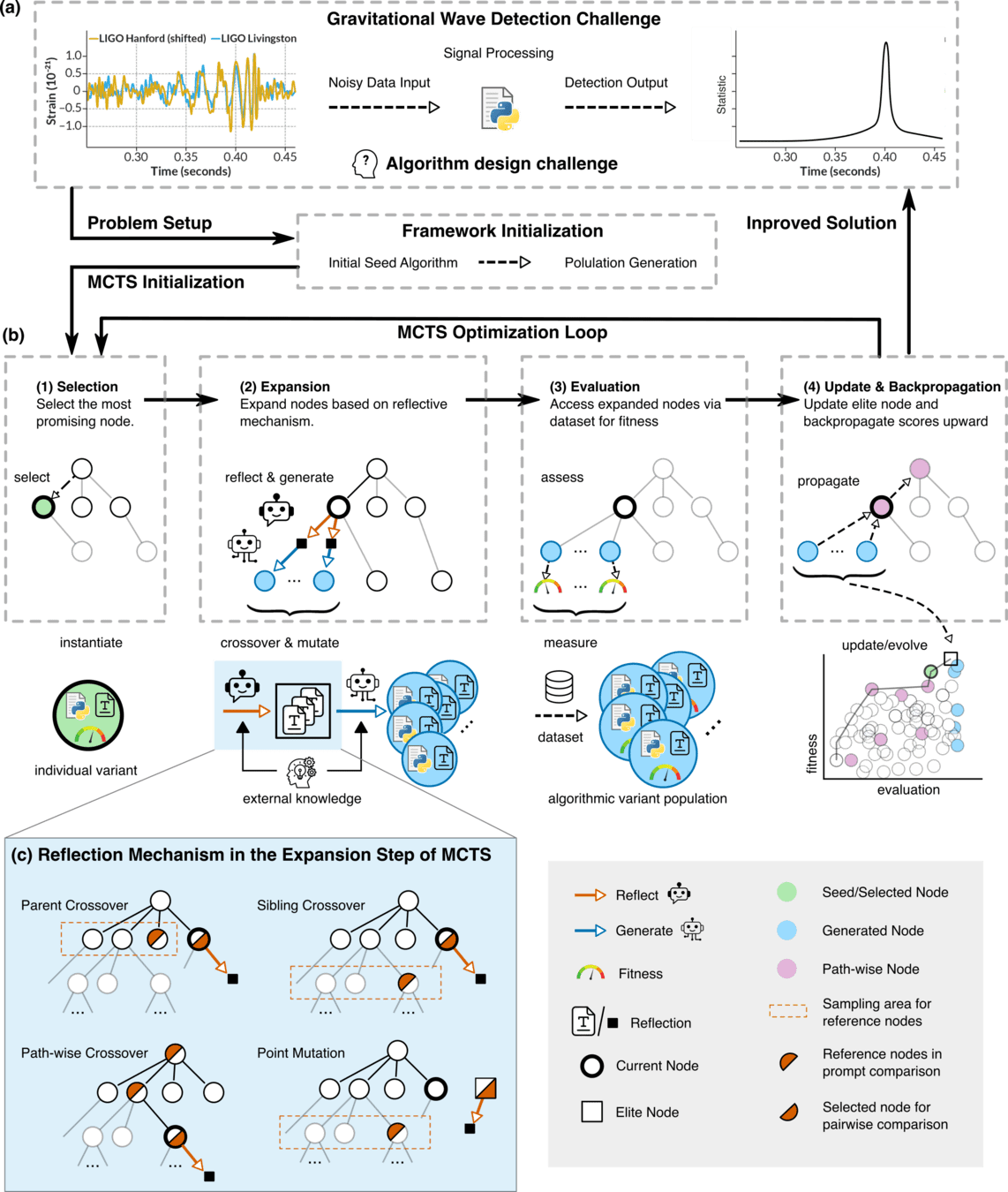
# Evo-MCTS
The LLM does not predict answers — it reshapes how we search for algorithms.
External evaluator: MLGWSC-1
Concept
Mechanism
Problem → Algorithm
Benchmark → Algorithm → Fitness
↻ LLM-guided search and refinement
From solving instances to discovering reusable methods
HW, LZ. arXiv:2508.03661 [cs.AI]
From solving instances to discovering reusable methods
# Evo-MCTS
The LLM does not predict answers — it reshapes how we search for algorithms.
external_knowledge
(constraint)
Execute on benchmark data
LLM as designer
arXiv:2410.14716 [cs.LG]
import numpy as np
import scipy.signal as signal
def pipeline_v1(strain_h1: np.ndarray, strain_l1: np.ndarray, times: np.ndarray) -> tuple[np.ndarray, np.ndarray, np.ndarray]:
    def data_conditioning(strain_h1: np.ndarray, strain_l1: np.ndarray, times: np.ndarray) -> tuple[np.ndarray, np.ndarray, np.ndarray]:
        window_length = 4096
        dt = times[1] - times[0]
        fs = 1.0 / dt

        def whiten_strain(strain):
            strain_zeromean = strain - np.mean(strain)
            freqs, psd = signal.welch(strain_zeromean, fs=fs, nperseg=window_length,
                                       window='hann', noverlap=window_length//2)
            smoothed_psd = np.convolve(psd, np.ones(32) / 32, mode='same')
            smoothed_psd = np.maximum(smoothed_psd, np.finfo(float).tiny)
            white_fft = np.fft.rfft(strain_zeromean) / np.sqrt(np.interp(np.fft.rfftfreq(len(strain_zeromean), d=dt), freqs, smoothed_psd))
            return np.fft.irfft(white_fft)

        whitened_h1 = whiten_strain(strain_h1)
        whitened_l1 = whiten_strain(strain_l1)

        return whitened_h1, whitened_l1, times

    def compute_metric_series(h1_data: np.ndarray, l1_data: np.ndarray, time_series: np.ndarray) -> tuple[np.ndarray, np.ndarray]:
        fs = 1 / (time_series[1] - time_series[0])
        f_h1, t_h1, Sxx_h1 = signal.spectrogram(h1_data, fs=fs, nperseg=256, noverlap=128, mode='magnitude', detrend=False)
        f_l1, t_l1, Sxx_l1 = signal.spectrogram(l1_data, fs=fs, nperseg=256, noverlap=128, mode='magnitude', detrend=False)
        tf_metric = np.mean((Sxx_h1**2 + Sxx_l1**2) / 2, axis=0)
        gps_mid_time = time_series[0] + (time_series[-1] - time_series[0]) / 2
        metric_times = gps_mid_time + (t_h1 - t_h1[-1] / 2)

        return tf_metric, metric_times

    def calculate_statistics(tf_metric, t_h1):
        background_level = np.median(tf_metric)
        peaks, _ = signal.find_peaks(tf_metric, height=background_level * 1.0, distance=2, prominence=background_level * 0.3)
        peak_times = t_h1[peaks]
        peak_heights = tf_metric[peaks]
        peak_deltat = np.full(len(peak_times), 10.0)  # Fixed uncertainty value
        return peak_times, peak_heights, peak_deltat

    whitened_h1, whitened_l1, data_times = data_conditioning(strain_h1, strain_l1, times)
    tf_metric, metric_times = compute_metric_series(whitened_h1, whitened_l1, data_times)
    peak_times, peak_heights, peak_deltat = calculate_statistics(tf_metric, metric_times)

    return peak_times, peak_heights, peak_deltat
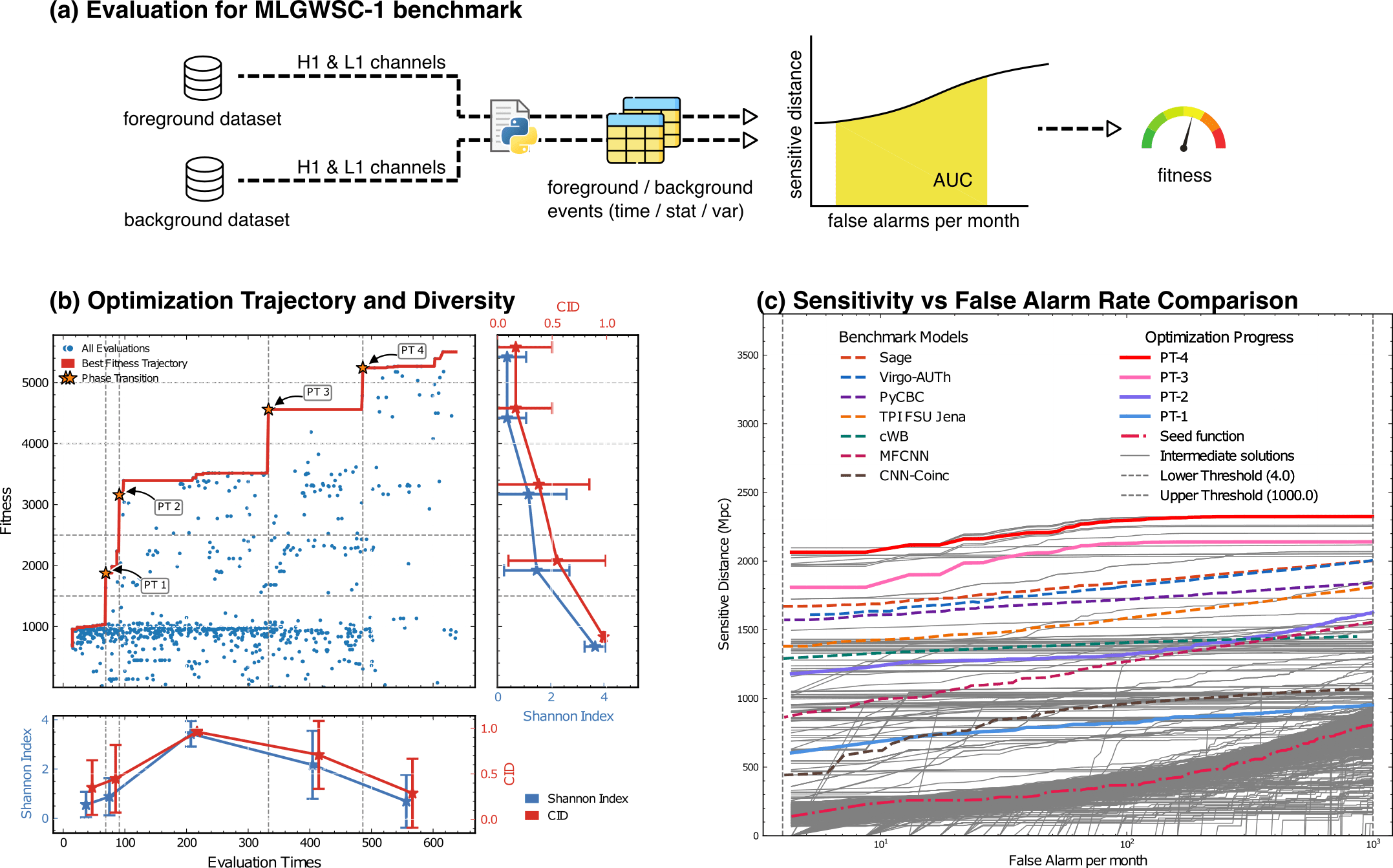
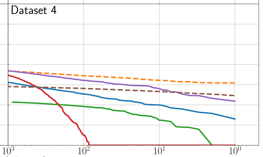
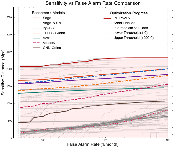
Optimization Target: Maximizing Area Under Curve (AUC) over the target false-alarm-rate range (e.g. 1–1000 false alarms/month), balancing detection sensitivity and false alarm rates across algorithm generations
MLGWSC-1 benchmark
HW, LZ. arXiv:2508.03661 [cs.AI]
# Evo-MCTS
The LLM does not predict answers — it reshapes how we search for algorithms.
external_knowledge
(constraint)
Execute on benchmark data
LLM as designer
arXiv:2410.14716 [cs.LG]
import numpy as np
import scipy.signal as signal
def pipeline_v1(strain_h1: np.ndarray, strain_l1: np.ndarray, times: np.ndarray) -> tuple[np.ndarray, np.ndarray, np.ndarray]:
    def data_conditioning(strain_h1: np.ndarray, strain_l1: np.ndarray, times: np.ndarray) -> tuple[np.ndarray, np.ndarray, np.ndarray]:
        window_length = 4096
        dt = times[1] - times[0]
        fs = 1.0 / dt

        def whiten_strain(strain):
            strain_zeromean = strain - np.mean(strain)
            freqs, psd = signal.welch(strain_zeromean, fs=fs, nperseg=window_length,
                                       window='hann', noverlap=window_length//2)
            smoothed_psd = np.convolve(psd, np.ones(32) / 32, mode='same')
            smoothed_psd = np.maximum(smoothed_psd, np.finfo(float).tiny)
            white_fft = np.fft.rfft(strain_zeromean) / np.sqrt(np.interp(np.fft.rfftfreq(len(strain_zeromean), d=dt), freqs, smoothed_psd))
            return np.fft.irfft(white_fft)

        whitened_h1 = whiten_strain(strain_h1)
        whitened_l1 = whiten_strain(strain_l1)

        return whitened_h1, whitened_l1, times

    def compute_metric_series(h1_data: np.ndarray, l1_data: np.ndarray, time_series: np.ndarray) -> tuple[np.ndarray, np.ndarray]:
        fs = 1 / (time_series[1] - time_series[0])
        f_h1, t_h1, Sxx_h1 = signal.spectrogram(h1_data, fs=fs, nperseg=256, noverlap=128, mode='magnitude', detrend=False)
        f_l1, t_l1, Sxx_l1 = signal.spectrogram(l1_data, fs=fs, nperseg=256, noverlap=128, mode='magnitude', detrend=False)
        tf_metric = np.mean((Sxx_h1**2 + Sxx_l1**2) / 2, axis=0)
        gps_mid_time = time_series[0] + (time_series[-1] - time_series[0]) / 2
        metric_times = gps_mid_time + (t_h1 - t_h1[-1] / 2)

        return tf_metric, metric_times

    def calculate_statistics(tf_metric, t_h1):
        background_level = np.median(tf_metric)
        peaks, _ = signal.find_peaks(tf_metric, height=background_level * 1.0, distance=2, prominence=background_level * 0.3)
        peak_times = t_h1[peaks]
        peak_heights = tf_metric[peaks]
        peak_deltat = np.full(len(peak_times), 10.0)  # Fixed uncertainty value
        return peak_times, peak_heights, peak_deltat

    whitened_h1, whitened_l1, data_times = data_conditioning(strain_h1, strain_l1, times)
    tf_metric, metric_times = compute_metric_series(whitened_h1, whitened_l1, data_times)
    peak_times, peak_heights, peak_deltat = calculate_statistics(tf_metric, metric_times)

    return peak_times, peak_heights, peak_deltat
HW, LZ. arXiv:2508.03661 [cs.AI]
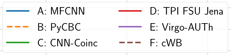
PyCBC (linear-core)
cWB (nonlinear-core)
Simple filters (non-linear)
CNN-like (highly non-linear)
Benchmarking against state-of-the-art methods
# Evo-MCTS
The LLM does not predict answers — it reshapes how we search for algorithms.
external_knowledge
(constraint)
Execute on benchmark data
LLM as designer
arXiv:2410.14716 [cs.LG]
import numpy as np
import scipy.signal as signal
def pipeline_v1(strain_h1: np.ndarray, strain_l1: np.ndarray, times: np.ndarray) -> tuple[np.ndarray, np.ndarray, np.ndarray]:
    def data_conditioning(strain_h1: np.ndarray, strain_l1: np.ndarray, times: np.ndarray) -> tuple[np.ndarray, np.ndarray, np.ndarray]:
        window_length = 4096
        dt = times[1] - times[0]
        fs = 1.0 / dt

        def whiten_strain(strain):
            strain_zeromean = strain - np.mean(strain)
            freqs, psd = signal.welch(strain_zeromean, fs=fs, nperseg=window_length,
                                       window='hann', noverlap=window_length//2)
            smoothed_psd = np.convolve(psd, np.ones(32) / 32, mode='same')
            smoothed_psd = np.maximum(smoothed_psd, np.finfo(float).tiny)
            white_fft = np.fft.rfft(strain_zeromean) / np.sqrt(np.interp(np.fft.rfftfreq(len(strain_zeromean), d=dt), freqs, smoothed_psd))
            return np.fft.irfft(white_fft)

        whitened_h1 = whiten_strain(strain_h1)
        whitened_l1 = whiten_strain(strain_l1)

        return whitened_h1, whitened_l1, times

    def compute_metric_series(h1_data: np.ndarray, l1_data: np.ndarray, time_series: np.ndarray) -> tuple[np.ndarray, np.ndarray]:
        fs = 1 / (time_series[1] - time_series[0])
        f_h1, t_h1, Sxx_h1 = signal.spectrogram(h1_data, fs=fs, nperseg=256, noverlap=128, mode='magnitude', detrend=False)
        f_l1, t_l1, Sxx_l1 = signal.spectrogram(l1_data, fs=fs, nperseg=256, noverlap=128, mode='magnitude', detrend=False)
        tf_metric = np.mean((Sxx_h1**2 + Sxx_l1**2) / 2, axis=0)
        gps_mid_time = time_series[0] + (time_series[-1] - time_series[0]) / 2
        metric_times = gps_mid_time + (t_h1 - t_h1[-1] / 2)

        return tf_metric, metric_times

    def calculate_statistics(tf_metric, t_h1):
        background_level = np.median(tf_metric)
        peaks, _ = signal.find_peaks(tf_metric, height=background_level * 1.0, distance=2, prominence=background_level * 0.3)
        peak_times = t_h1[peaks]
        peak_heights = tf_metric[peaks]
        peak_deltat = np.full(len(peak_times), 10.0)  # Fixed uncertainty value
        return peak_times, peak_heights, peak_deltat

    whitened_h1, whitened_l1, data_times = data_conditioning(strain_h1, strain_l1, times)
    tf_metric, metric_times = compute_metric_series(whitened_h1, whitened_l1, data_times)
    peak_times, peak_heights, peak_deltat = calculate_statistics(tf_metric, metric_times)

    return peak_times, peak_heights, peak_deltat
HW, LZ. arXiv:2508.03661 [cs.AI]
PyCBC (linear-core)
cWB (nonlinear-core)
Simple filters (non-linear)
CNN-like (highly non-linear)
Benchmarking against state-of-the-art methods
# Evo-MCTS
The LLM does not predict answers — it reshapes how we search for algorithms.
external_knowledge
(constraint)
LLM as designer
arXiv:2410.14716 [cs.LG]
HW, LZ. arXiv:2508.03661 [cs.AI]
You are an expert in gravitational wave signal detection algorithms. Your task is to design heuristics that can effectively solve optimization problems.

{prompt_task}

I have analyzed two algorithms and provided a reflection on their differences.

[Worse code]
{worse_code}

[Better code]
{better_code}

[Reflection]
{reflection}

{external_knowledge}

Based on this reflection, please write an improved algorithm according to the reflection.
First, describe the design idea and main steps of your algorithm in one sentence. The description must be inside a brace outside the code implementation. Next, implement it in Python as a function named '{func_name}'.
This function should accept {input_count} input(s): {joined_inputs}. The function should return {output_count} output(s): {joined_outputs}.
{inout_inf} {other_inf}

Do not give additional explanations.
One Prompt Template for MLGWSC1 Algorithm Synthesis
# Evo-MCTS
Tree search over LLM-generated algorithms
external_knowledge
(constraint)
LLM as designer
arXiv:2410.14716 [cs.LG]
HW, LZ. arXiv:2508.03661 [cs.AI]
# Evo-MCTS
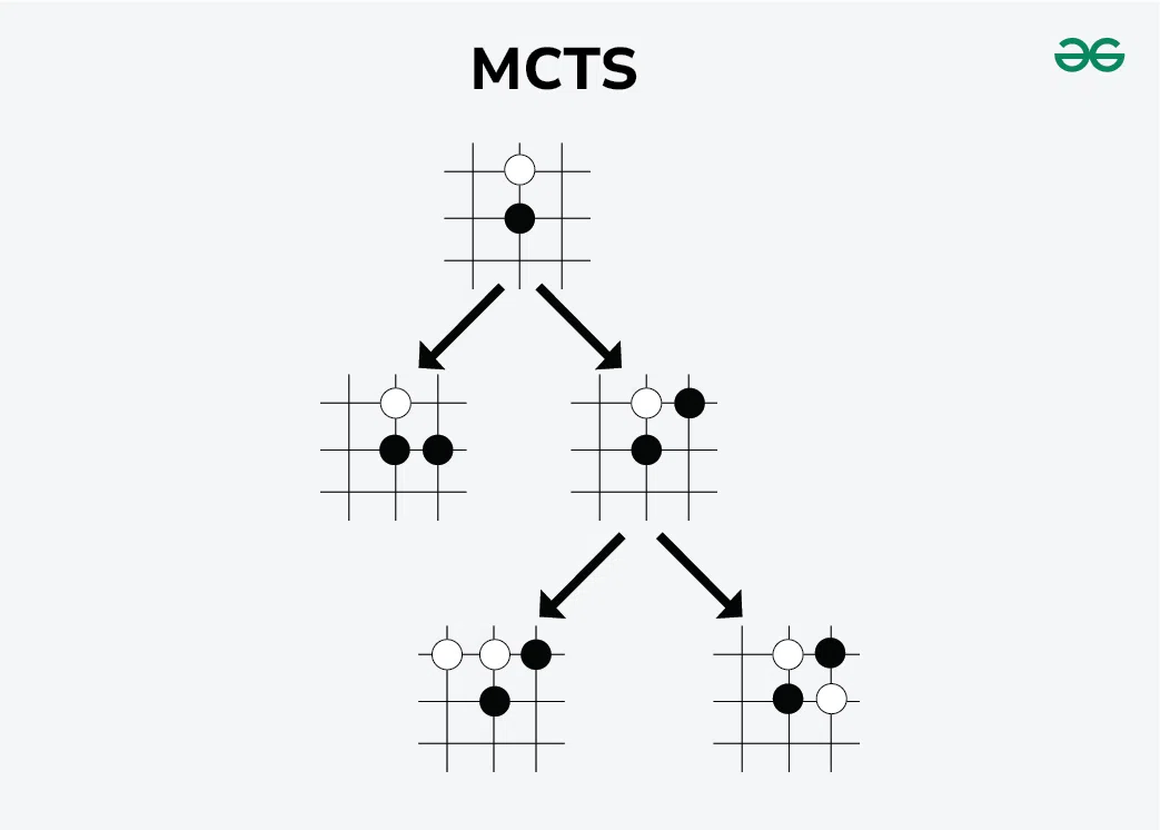
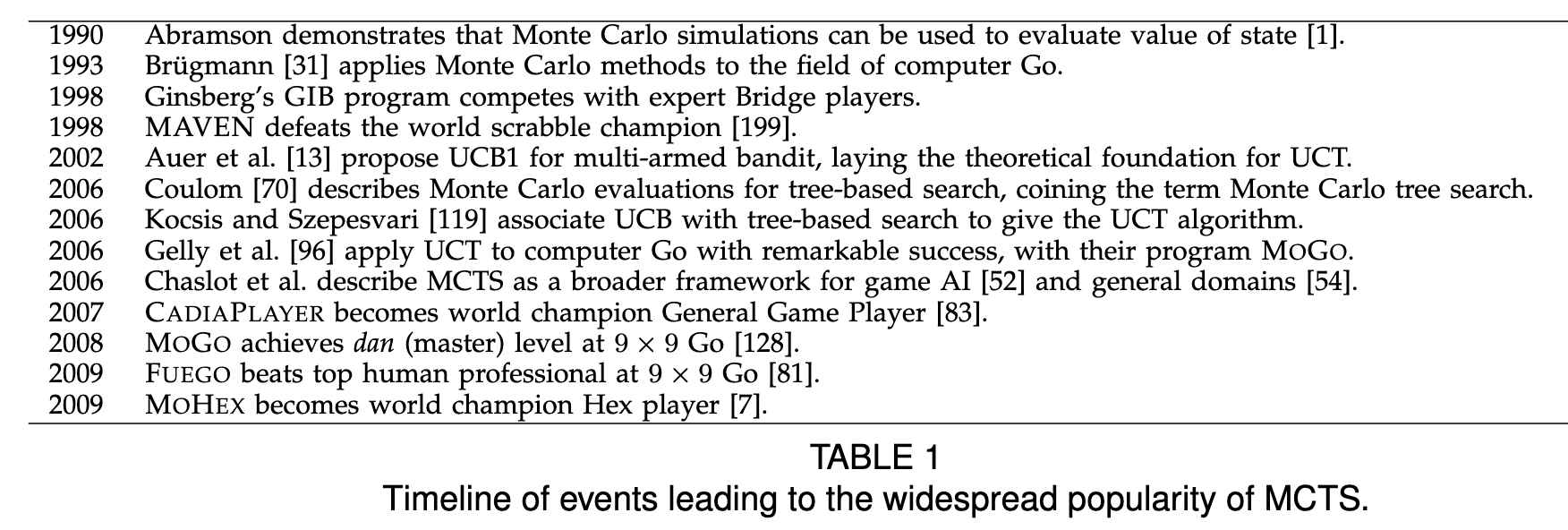
MCTS
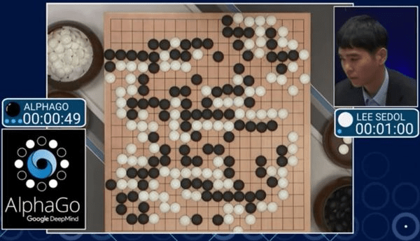
Casse1: Go Game
Case 2: Reasoning models and test-time compute
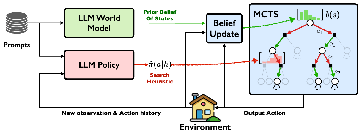
The release of o1 marks the formal deployment of the inference-time scaling paradigm in production. As Richard Sutton pointed out in The Bitter Lesson, only learning and search are methods that can scale indefinitely with compute. From this point on, the focus has increasingly shifted toward search.
Browne et al. (2012)
arXiv:2305.14078 [cs.RO]
Monte Carlo Tree Search (MCTS), which allocates computation to promising branches while preserving exploration, has long been a core technique in modern game-playing systems such as AlphaGo.
LLM-Informed Evo-MCTS
# Evo-MCTS
LLM-Informed Evo-MCTS
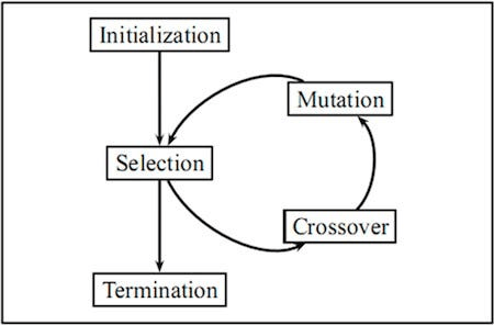
EA
Evolution proposes diverse variants; MCTS decides where to spend search budget.
Evolutionary Algorithms (EAs) provide:
They are especially natural when the search object is executable code.
Population-level search
# Evo-MCTS
The LLM does not predict answers — it reshapes how we search for algorithms.
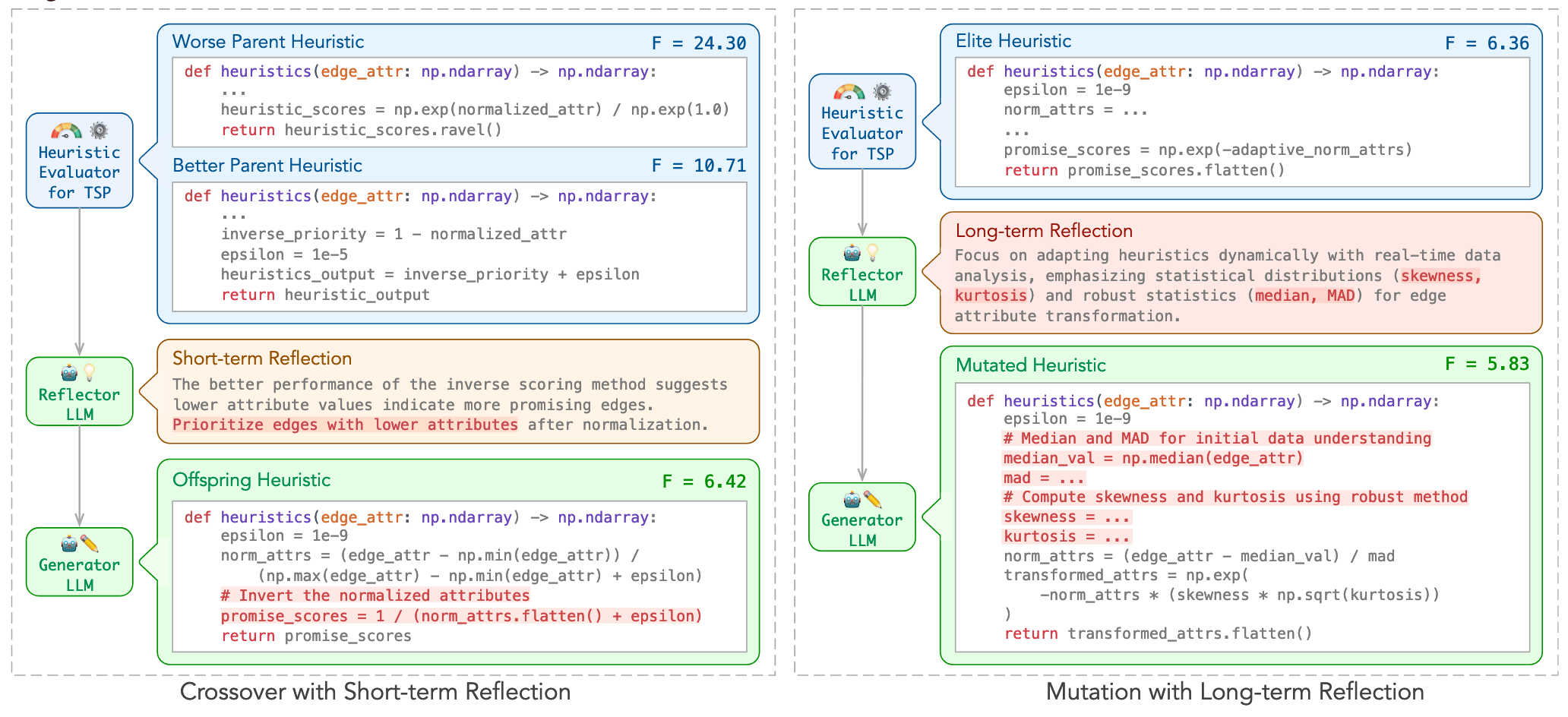
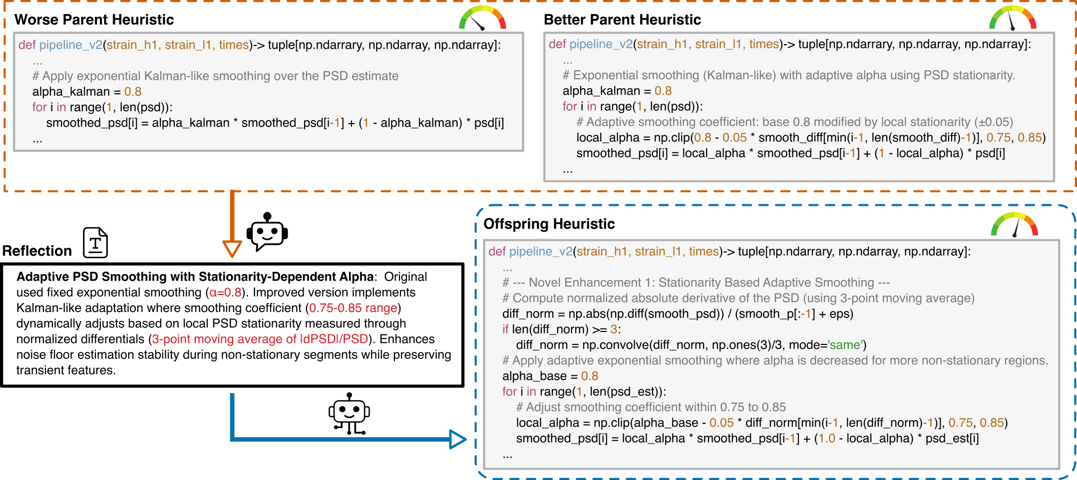
Reflection-Guided Code Evolution
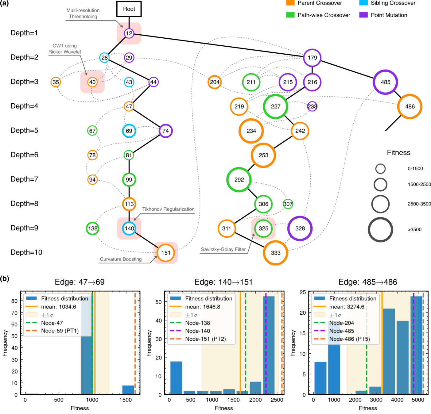
Evo-MCTS Search Trajectory
What changed?
LLMs propose actions that guide the search
Past evaluations become structured search memory
Search history conditions future algorithm generation
HW, LZ. arXiv:2508.03661 [cs.AI]
Compare → Reflect → Rewrite → Evaluate
# Evo-MCTS
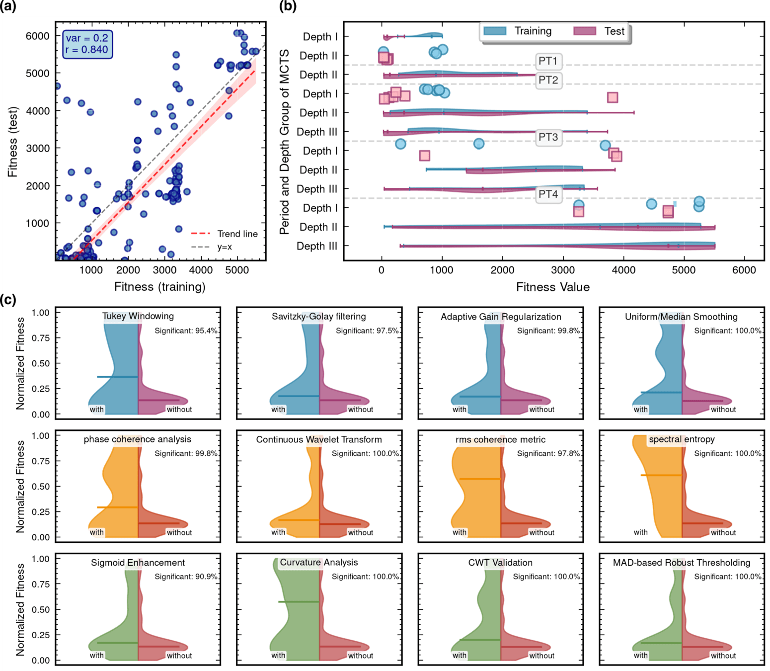
What did the discovered algorithm actually learn to do?
HW, LZ. arXiv:2508.03661 [cs.AI]
Algorithmic Component Impact Analysis.
import numpy as np
import scipy.signal as signal
from scipy.signal.windows import tukey
from scipy.signal import savgol_filter

def pipeline_v2(strain_h1: np.ndarray, strain_l1: np.ndarray, times: np.ndarray) -> tuple[np.ndarray, np.ndarray, np.ndarray]:
    """
    The pipeline function processes gravitational wave data from the H1 and L1 detectors to identify potential gravitational wave signals.
    It takes strain_h1 and strain_l1 numpy arrays containing detector data, and times array with corresponding time points.
    The function returns a tuple of three numpy arrays: peak_times containing GPS times of identified events,
    peak_heights with significance values of each peak, and peak_deltat showing time window uncertainty for each peak.
    """
    eps = np.finfo(float).tiny
    dt = times[1] - times[0]
    fs = 1.0 / dt
    # Base spectrogram parameters
    base_nperseg = 256
    base_noverlap = base_nperseg // 2
    medfilt_kernel = 101       # odd kernel size for robust detrending
    uncertainty_window = 5     # half-window for local timing uncertainty

    # -------------------- Stage 1: Robust Baseline Detrending --------------------
    # Remove long-term trends using a median filter for each channel.
    detrended_h1 = strain_h1 - signal.medfilt(strain_h1, kernel_size=medfilt_kernel)
    detrended_l1 = strain_l1 - signal.medfilt(strain_l1, kernel_size=medfilt_kernel)

    # -------------------- Stage 2: Adaptive Whitening with Enhanced PSD Smoothing --------------------
    def adaptive_whitening(strain: np.ndarray) -> np.ndarray:
        # Center the signal.
        centered = strain - np.mean(strain)
        n_samples = len(centered)
        # Adaptive window length: between 5 and 30 seconds
        win_length_sec = np.clip(n_samples / fs / 20, 5, 30)
        nperseg_adapt = int(win_length_sec * fs)
        nperseg_adapt = max(10, min(nperseg_adapt, n_samples))

        # Create a Tukey window with 75% overlap.
        tukey_alpha = 0.25
        win = tukey(nperseg_adapt, alpha=tukey_alpha)
        noverlap_adapt = int(nperseg_adapt * 0.75)
        if noverlap_adapt >= nperseg_adapt:
            noverlap_adapt = nperseg_adapt - 1

        # Estimate the power spectral density (PSD) using Welch's method.
        freqs, psd = signal.welch(centered, fs=fs, nperseg=nperseg_adapt,
                                  noverlap=noverlap_adapt, window=win, detrend='constant')
        psd = np.maximum(psd, eps)

        # Compute relative differences for PSD stationarity measure.
        diff_arr = np.abs(np.diff(psd)) / (psd[:-1] + eps)
        # Smooth the derivative with a moving average.
        if len(diff_arr) >= 3:
            smooth_diff = np.convolve(diff_arr, np.ones(3)/3, mode='same')
        else:
            smooth_diff = diff_arr

        # Exponential smoothing (Kalman-like) with adaptive alpha using PSD stationarity.
        smoothed_psd = np.copy(psd)
        for i in range(1, len(psd)):
            # Adaptive smoothing coefficient: base 0.8 modified by local stationarity (±0.05)
            local_alpha = np.clip(0.8 - 0.05 * smooth_diff[min(i-1, len(smooth_diff)-1)], 0.75, 0.85)
            smoothed_psd[i] = local_alpha * smoothed_psd[i-1] + (1 - local_alpha) * psd[i]

        # Compute Tikhonov regularization gain based on deviation from median PSD.
        noise_baseline = np.median(smoothed_psd)
        raw_gain = (smoothed_psd / (noise_baseline + eps)) - 1.0

        # Compute a causal-like gradient using the Savitzky-Golay filter.
        win_len = 11 if len(smoothed_psd) >= 11 else ((len(smoothed_psd)//2)*2+1)
        polyorder = 2 if win_len > 2 else 1
        delta_freq = np.mean(np.diff(freqs))
        grad_psd = savgol_filter(smoothed_psd, win_len, polyorder, deriv=1, delta=delta_freq, mode='interp')

        # Nonlinear scaling via sigmoid to enhance gradient differences.
        sigmoid = lambda x: 1.0 / (1.0 + np.exp(-x))
        scaling_factor = 1.0 + 2.0 * sigmoid(np.abs(grad_psd) / (np.median(smoothed_psd) + eps))

        # Compute adaptive gain factors with nonlinear scaling.
        gain = 1.0 - np.exp(-0.5 * scaling_factor * raw_gain)
        gain = np.clip(gain, -8.0, 8.0)

        # FFT-based whitening: interpolate gain and PSD onto FFT frequency bins.
        signal_fft = np.fft.rfft(centered)
        freq_bins = np.fft.rfftfreq(n_samples, d=dt)
        interp_gain = np.interp(freq_bins, freqs, gain, left=gain[0], right=gain[-1])
        interp_psd = np.interp(freq_bins, freqs, smoothed_psd, left=smoothed_psd[0], right=smoothed_psd[-1])
        denom = np.sqrt(interp_psd) * (np.abs(interp_gain) + eps)
        denom = np.maximum(denom, eps)
        white_fft = signal_fft / denom
        whitened = np.fft.irfft(white_fft, n=n_samples)
        return whitened

    # Whiten H1 and L1 channels using the adapted method.
    white_h1 = adaptive_whitening(detrended_h1)
    white_l1 = adaptive_whitening(detrended_l1)

    # -------------------- Stage 3: Coherent Time-Frequency Metric with Frequency-Conditioned Regularization --------------------
    def compute_coherent_metric(w1: np.ndarray, w2: np.ndarray) -> tuple[np.ndarray, np.ndarray]:
        # Compute complex spectrograms preserving phase information.
        f1, t_spec, Sxx1 = signal.spectrogram(w1, fs=fs, nperseg=base_nperseg,
                                              noverlap=base_noverlap, mode='complex', detrend=False)
        f2, t_spec2, Sxx2 = signal.spectrogram(w2, fs=fs, nperseg=base_nperseg,
                                               noverlap=base_noverlap, mode='complex', detrend=False)
        # Ensure common time axis length.
        common_len = min(len(t_spec), len(t_spec2))
        t_spec = t_spec[:common_len]
        Sxx1 = Sxx1[:, :common_len]
        Sxx2 = Sxx2[:, :common_len]

        # Compute phase differences and coherence between detectors.
        phase_diff = np.angle(Sxx1) - np.angle(Sxx2)
        phase_coherence = np.abs(np.cos(phase_diff))

        # Estimate median PSD per frequency bin from the spectrograms.
        psd1 = np.median(np.abs(Sxx1)**2, axis=1)
        psd2 = np.median(np.abs(Sxx2)**2, axis=1)

        # Frequency-conditioned regularization gain (reflection-guided).
        lambda_f = 0.5 * ((np.median(psd1) / (psd1 + eps)) + (np.median(psd2) / (psd2 + eps)))
        lambda_f = np.clip(lambda_f, 1e-4, 1e-2)
        # Regularization denominator integrating detector PSDs and lambda.
        reg_denom = (psd1[:, None] + psd2[:, None] + lambda_f[:, None] + eps)

        # Weighted phase coherence that balances phase alignment with noise levels.
        weighted_comp = phase_coherence / reg_denom

        # Compute axial (frequency) second derivatives as curvature estimates.
        d2_coh = np.gradient(np.gradient(phase_coherence, axis=0), axis=0)
        avg_curvature = np.mean(np.abs(d2_coh), axis=0)

        # Nonlinear activation boost using tanh for regions of high curvature.
        nonlinear_boost = np.tanh(5 * avg_curvature)
        linear_boost = 1.0 + 0.1 * avg_curvature

        # Cross-detector synergy: weight derived from global median consistency.
        novel_weight = np.mean((np.median(psd1) + np.median(psd2)) / (psd1[:, None] + psd2[:, None] + eps), axis=0)

        # Integrated time-frequency metric combining all enhancements.
        tf_metric = np.sum(weighted_comp * linear_boost * (1.0 + nonlinear_boost), axis=0) * novel_weight

        # Adjust the spectrogram time axis to account for window delay.
        metric_times = t_spec + times[0] + (base_nperseg / 2) / fs
        return tf_metric, metric_times

    tf_metric, metric_times = compute_coherent_metric(white_h1, white_l1)

    # -------------------- Stage 4: Multi-Resolution Thresholding with Octave-Spaced Dyadic Wavelet Validation --------------------
    def multi_resolution_thresholding(metric: np.ndarray, times_arr: np.ndarray) -> tuple[np.ndarray, np.ndarray, np.ndarray]:
        # Robust background estimation with median and MAD.
        bg_level = np.median(metric)
        mad_val = np.median(np.abs(metric - bg_level))
        robust_std = 1.4826 * mad_val
        threshold = bg_level + 1.5 * robust_std

        # Identify candidate peaks using prominence and minimum distance criteria.
        peaks, _ = signal.find_peaks(metric, height=threshold, distance=2, prominence=0.8 * robust_std)
        if peaks.size == 0:
            return np.array([]), np.array([]), np.array([])

        # Local uncertainty estimation using a Gaussian-weighted convolution.
        win_range = np.arange(-uncertainty_window, uncertainty_window + 1)
        sigma = uncertainty_window / 2.5
        gauss_kernel = np.exp(-0.5 * (win_range / sigma) ** 2)
        gauss_kernel /= np.sum(gauss_kernel)
        weighted_mean = np.convolve(metric, gauss_kernel, mode='same')
        weighted_sq = np.convolve(metric ** 2, gauss_kernel, mode='same')
        variances = np.maximum(weighted_sq - weighted_mean ** 2, 0.0)
        uncertainties = np.sqrt(variances)
        uncertainties = np.maximum(uncertainties, 0.01)

        valid_times = []
        valid_heights = []
        valid_uncerts = []
        n_metric = len(metric)

        # Compute a simple second derivative for local curvature checking.
        if n_metric > 2:
            second_deriv = np.diff(metric, n=2)
            second_deriv = np.pad(second_deriv, (1, 1), mode='edge')
        else:
            second_deriv = np.zeros_like(metric)

        # Use octave-spaced scales (dyadic wavelet validation) to validate peak significance.
        widths = np.arange(1, 9)  # approximate scales 1 to 8
        for peak in peaks:
            # Skip peaks lacking sufficient negative curvature.
            if second_deriv[peak] > -0.1 * robust_std:
                continue
            local_start = max(0, peak - uncertainty_window)
            local_end = min(n_metric, peak + uncertainty_window + 1)
            local_segment = metric[local_start:local_end]
            if len(local_segment) < 3:
                continue
            try:
                cwt_coeff = signal.cwt(local_segment, signal.ricker, widths)
            except Exception:
                continue
            max_coeff = np.max(np.abs(cwt_coeff))
            # Threshold for validating the candidate using local MAD.
            cwt_thresh = mad_val * np.sqrt(2 * np.log(len(local_segment) + eps))
            if max_coeff >= cwt_thresh:
                valid_times.append(times_arr[peak])
                valid_heights.append(metric[peak])
                valid_uncerts.append(uncertainties[peak])

        if len(valid_times) == 0:
            return np.array([]), np.array([]), np.array([])
        return np.array(valid_times), np.array(valid_heights), np.array(valid_uncerts)

    peak_times, peak_heights, peak_deltat = multi_resolution_thresholding(tf_metric, metric_times)
return peak_times, peak_heights, peak_deltat# Evo-MCTS
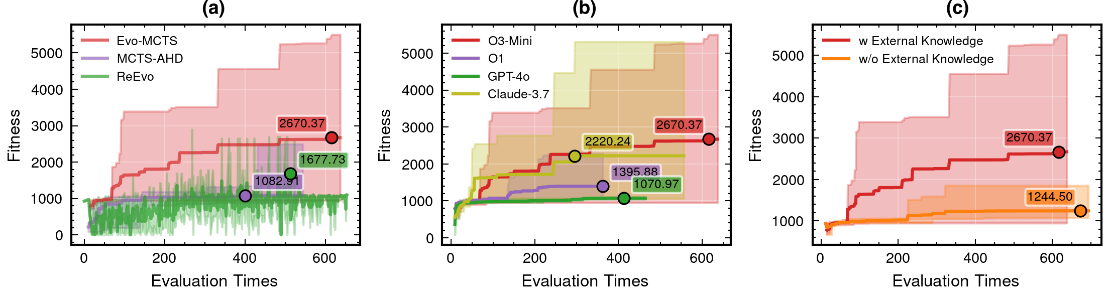
Architecture, model choice, and external knowledge each contribute differently.
HW, LZ. arXiv:2508.03661 [cs.AI]
1. Does the integrated search architecture matter?
3. Does prior scientific knowledge help?
2. How much does the choice of LLM matter?
o3-mini-medium
o1-2024-12-17
gpt-4o-2024-11-20
claude-3-7-sonnet-20250219-thinking
59.1% vs. best baseline
+115% with external knowledge
Full integration gives the strongest search trajectory and final fitness.
Search helps, but stronger reasoning/code models still produce better algorithmic proposals.
# Evo-MCTS
Architecture, model choice, and external knowledge each contribute differently.
HW, LZ. arXiv:2508.03661 [cs.AI]
1. Does the integrated search architecture matter?
3. Does prior scientific knowledge help?
2. How much does the choice of LLM matter?
o3-mini-medium
o1-2024-12-17
gpt-4o-2024-11-20
claude-3-7-sonnet-20250219-thinking
59.1% vs. best baseline
+115% with external knowledge
Full integration gives the strongest search trajectory and final fitness.
59.1%
### External Knowledge Integration
1. **Non-linear** Processing Core Concepts:
    - Signal Transformation:
        * Non-linear vs linear decomposition
        * Adaptive threshold mechanisms
        * Multi-scale analysis

    - Feature Extraction:
        * Phase space reconstruction
        * Topological data analysis
        * Wavelet-based detection

    - Statistical Analysis:
        * Robust estimators
        * Non-Gaussian processes
        * Higher-order statistics

2. Implementation Principles:
    - Prioritize adaptive over fixed parameters
    - Consider local vs global characteristics
- Balance computational cost with accuracy# Evo-MCTS
Scientific discovery requires interpretability — not just performance.
Interpretable AI Approach
The best of both worlds
Input
Physics-Informed
Algorithm
(High interpretability)
Output
Example: FunSearch,
Evo-MCTS, AlphaEvolve
AI Model
Physics
Knowledge
Traditional Physics Approach
Input
Human-Designed Algorithm
(Based on human insight)
Output
Example: Matched Filtering, linear regression
Black-Box AI Approach
Input
AI Model
(Low interpretability)
Output
Examples: CNN, AlphaGo, DINGO
Data/
Experience
Data/
Experience
🎯 OUR WORK
From predicting with AI to discovering algorithms with AI.
From interpolation to search, verification, and science
# Discovery
Scientific discovery requires interpretability — not just performance.
vs
Algorithm design can often be reframed as optimization in program space.
Many steps in gravitational-wave analysis can be treated similarly:
filter design · noise modeling · detection statistics · proposal mechanisms · inference strategies
The same perspective can extend to:
symbolic regression · analytic ansatz discovery · equation search · experimental design
# Discovery
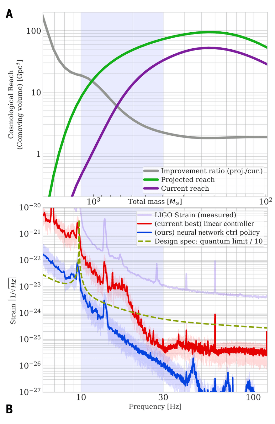
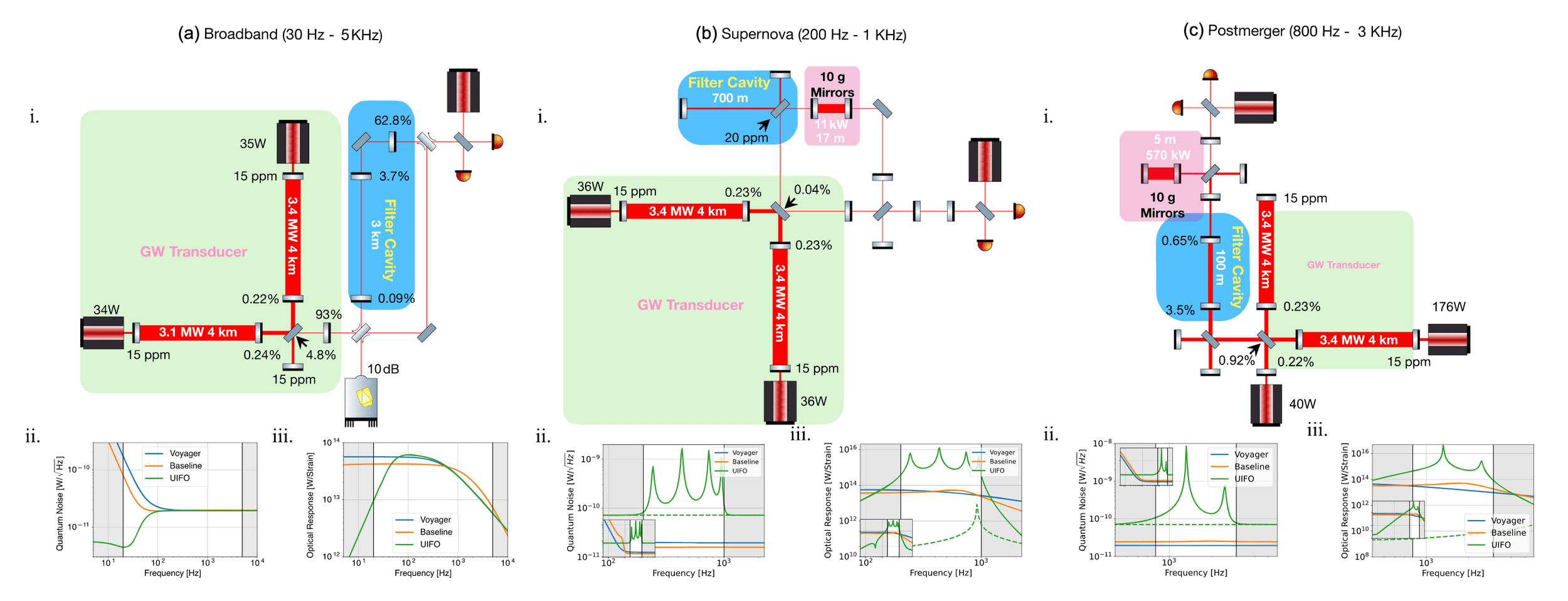
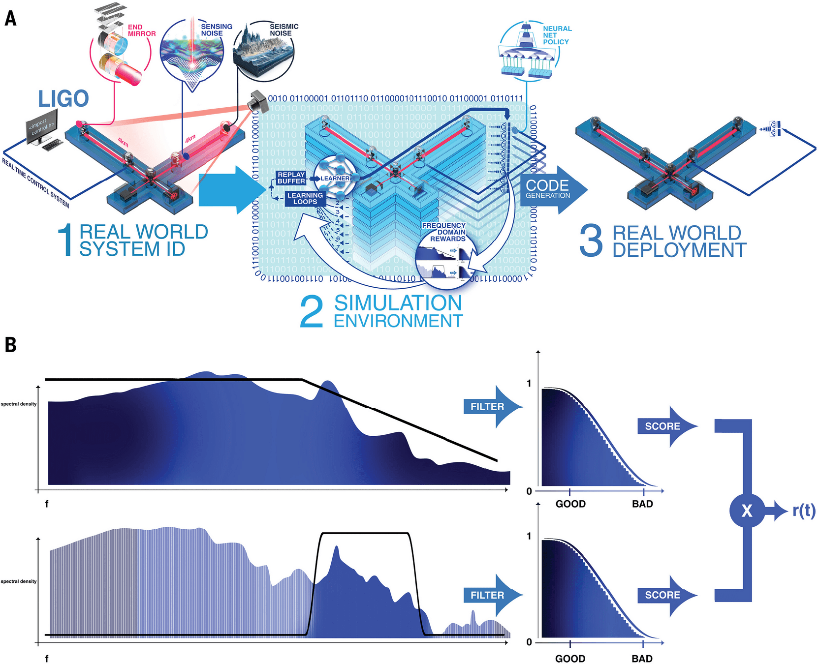
Scientific objects themselves can become optimization targets.
Phys. Rev. X 15, 021012 (2025)
Buchli+, Science (2025)
# Discovery
Is deep learning really discovering — or mostly interpolating?
Much of deep learning’s empirical success can be understood as powerful interpolation over learned representations.
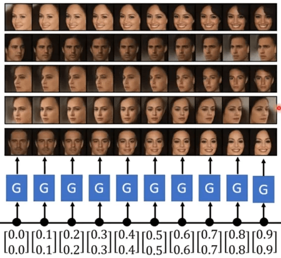
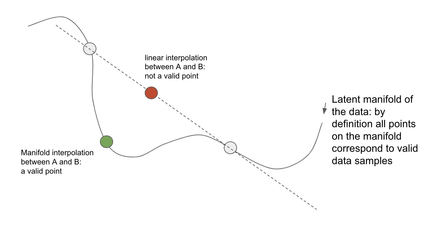
Interpolation in input space may be meaningless; interpolation in a learned latent space can be highly structured.
例如人脸 morph 的例子就很好:像素空间线性插值和 latent space 插值不是一回事。深度模型真正强的地方,往往是先把数据组织成一个有结构的 representation manifold,再在这个空间里做平滑泛化。
Deep Learning is Not As Impressive As you Think, It's Mere Interpolation (Source)
# Discovery
Is deep learning really discovering — or mostly interpolating?
Much of deep learning’s empirical success can be understood as powerful interpolation over learned representations.
Representation Space Interpolation
Representation Space Interpolation
Interpolation in input space may be meaningless; interpolation in a learned latent space can be highly structured.
例如人脸 morph 的例子就很好:像素空间线性插值和 latent space 插值不是一回事。深度模型真正强的地方,往往是先把数据组织成一个有结构的 representation manifold,再在这个空间里做平滑泛化。
Deep Learning is Not As Impressive As you Think, It's Mere Interpolation (Source)
# Discovery
The geometry of representation determines whether interpolation is meaningful.
Representation Space Interpolation
Deep learning 的强大之处,很多时候不是“凭空外推”,而是学到了一个 representation,使得原来复杂的数据关系在这个 manifold 空间里变得更平滑、更容易插值。
Deep Learning is Not As Impressive As you Think, It's Mere Interpolation (Source)
# Discovery
Generalization depends on how well data reveals the underlying representation space.
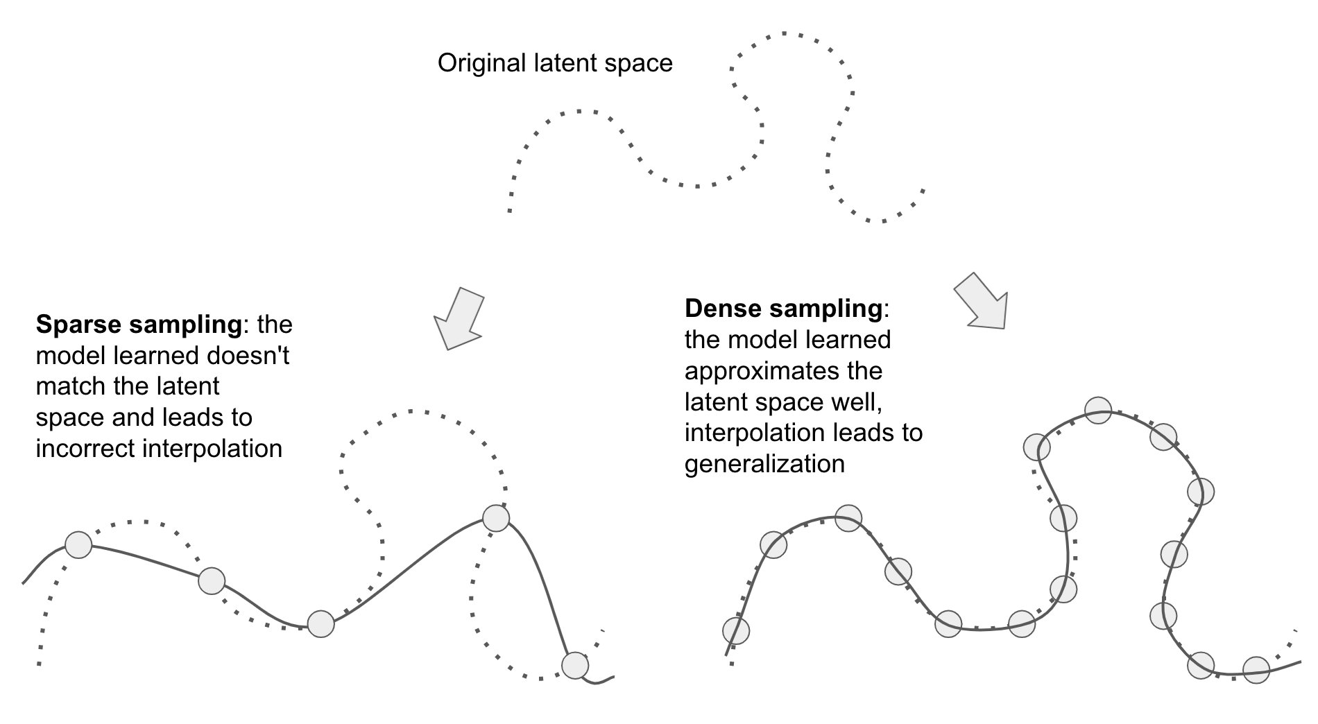
Generalization is not magic — it comes from structure shared between training and unseen data.
AI 之所以可以在“没见过”的样本上表现好,并不意味着它真的见到了一个完全陌生的世界。很多时候,新样本虽然没出现过,但仍然落在训练数据已经覆盖的同一个结构上。
Deep Learning is Not As Impressive As you Think, It's Mere Interpolation (Source)
Underlying data manifold / latent structure
也就是现实数据真正分布的“结构”。
Sparse data → wrong geometry → poor generalization
训练数据太稀疏时,模型只能从少量样本猜测这个结构,因此学到的 manifold 可能偏离真实 manifold。
Dense coverage → better representation → reliable interpolation
数据覆盖越充分,模型越容易学到接近真实 manifold 的表示,因此在已覆盖结构附近做 interpolation 时,泛化会更稳定。
LLMs appear highly general because their training distribution is extraordinarily broad.
GPT 看起来能回答一个“从没见过的问题”,不一定意味着它在严格数学意义上做了很远的 extrapolation;很可能是因为互联网规模的训练数据已经让 latent space 覆盖了极其丰富的语言、代码和知识结构。
所以,
# Discovery
What changes is not only the model — but the object being searched.
# Discovery
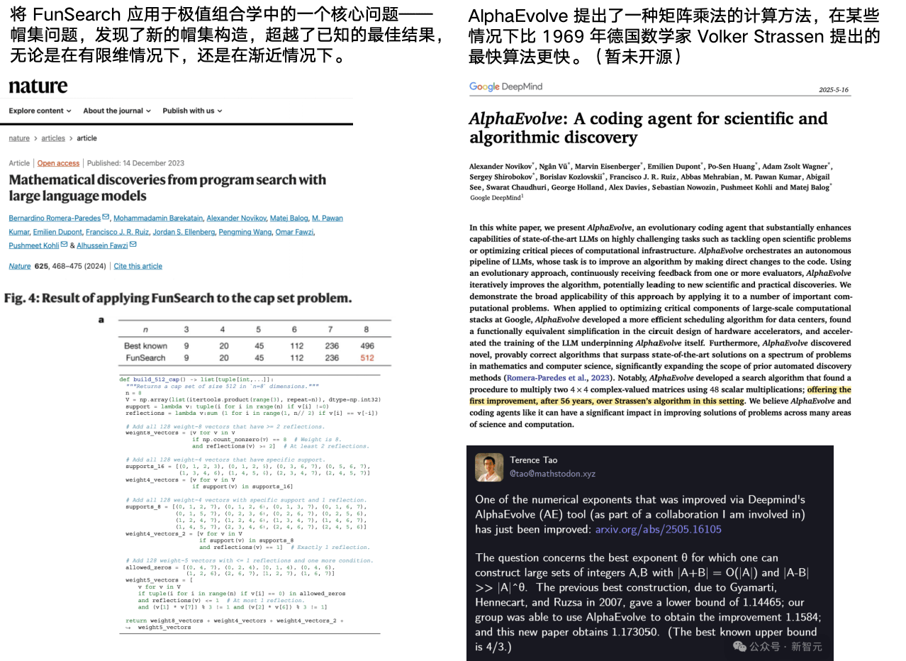
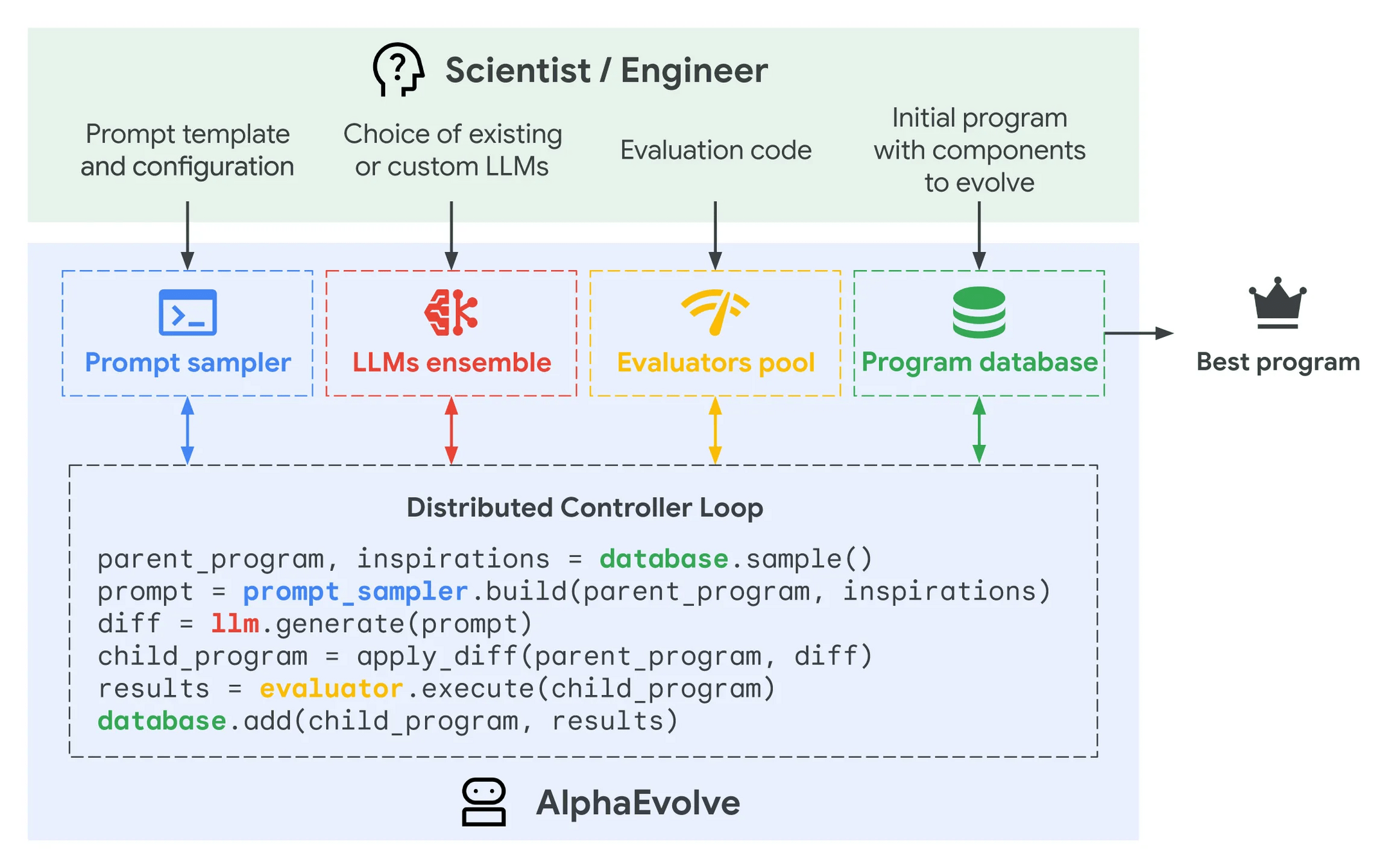
AlphaEvolve turns LLM proposals into verifiable algorithmic discoveries
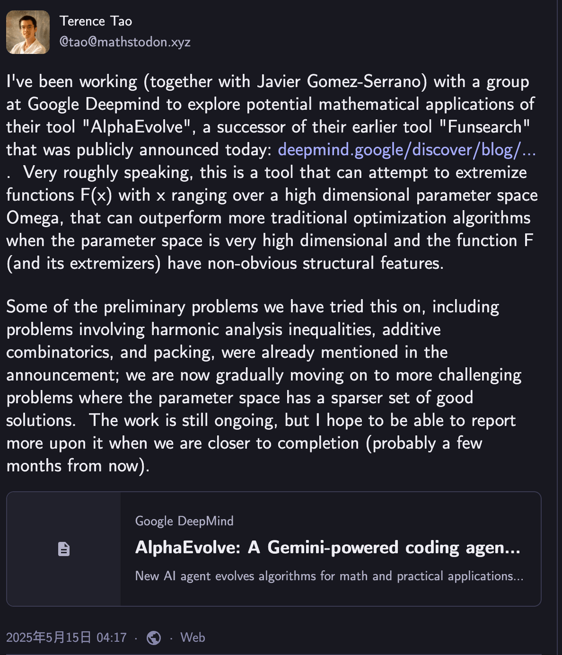
Tao’s perspective: AlphaEvolve is essentially trying to extremize complex high-dimensional functions when the good solutions are sparse and structured.
arXiv:2506.13131 [cs.AI]
# Discovery
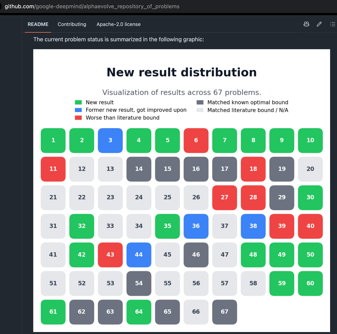
Terence Tao’s large-scale exploration across 67 mathematical problems
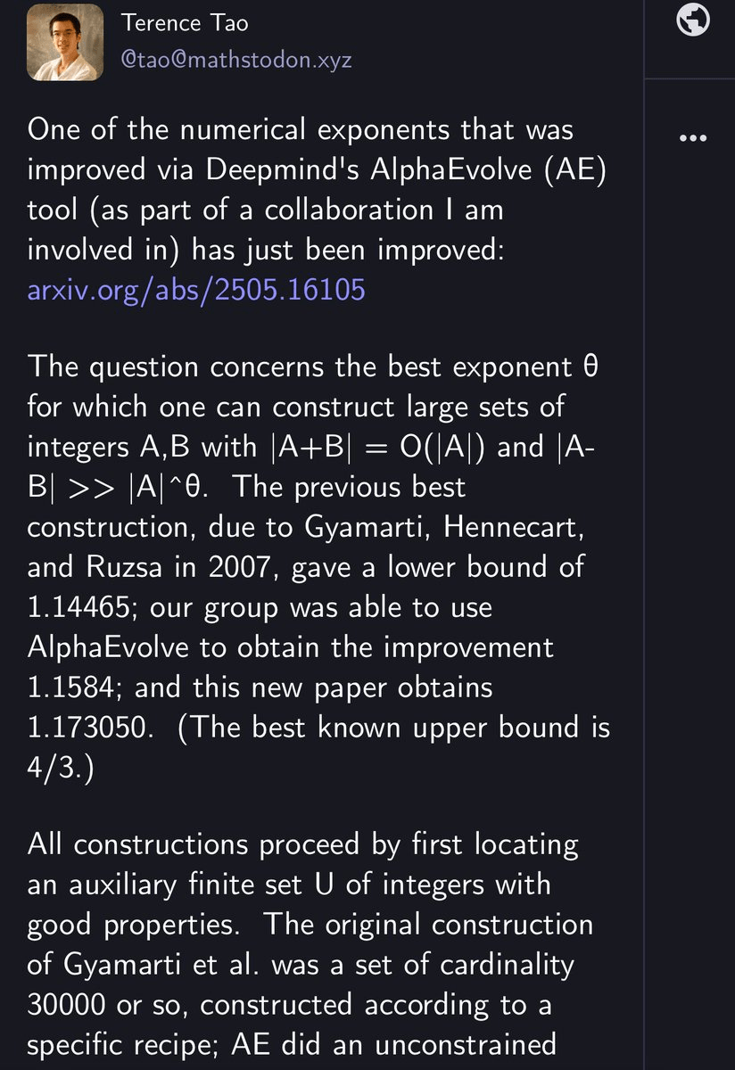
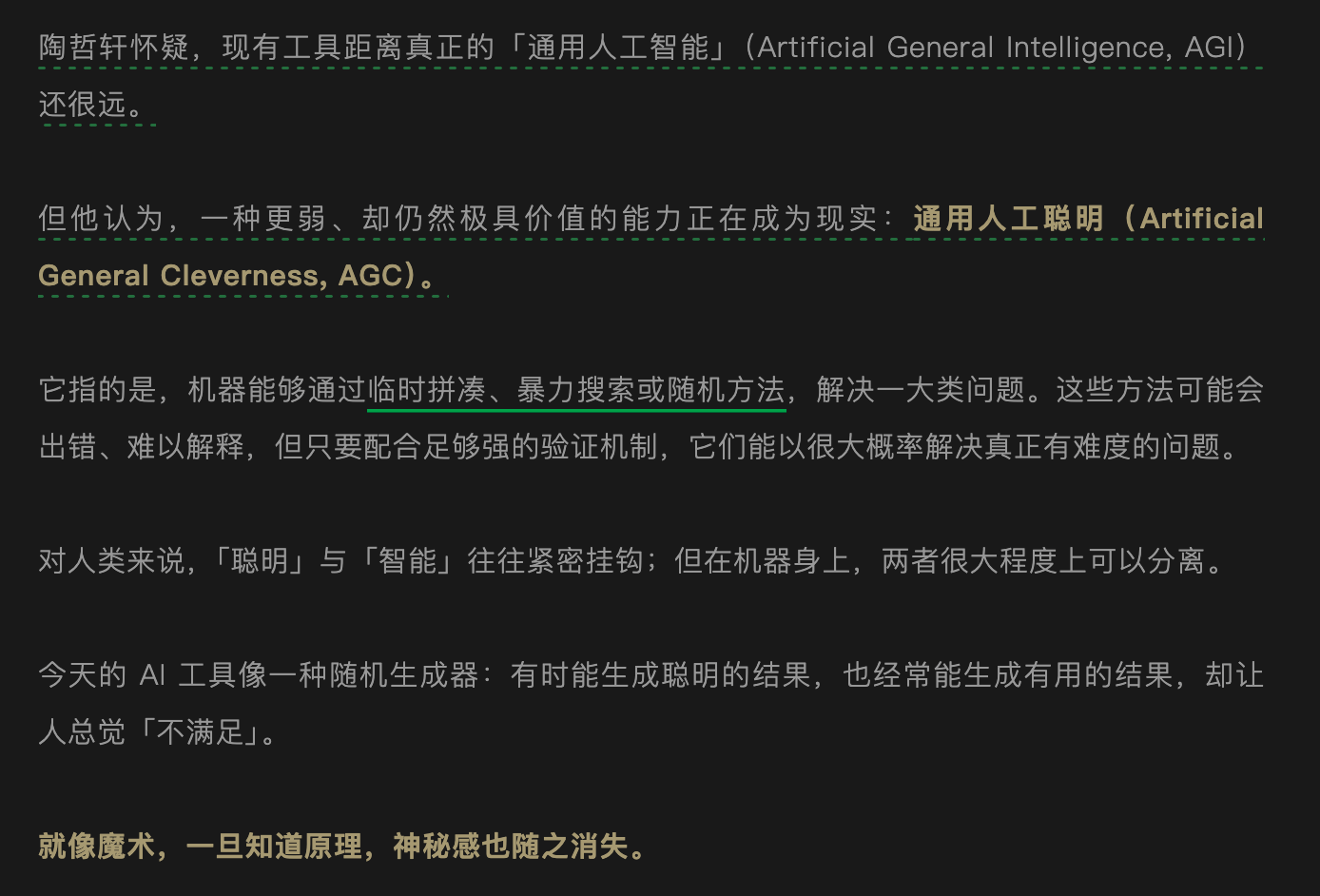
Tao 提到 sum-difference exponent :
\(1.14465 \rightarrow 1.1584 \rightarrow 1.173050\)
其中中间的提升来自 AlphaEvolve 相关探索,随后又被新的工作进一步提高。
Tao 提到,在 arithmetic Kakeya / sum-difference exponent 的探索中,AlphaEvolve 找到候选结构后,这些计算结果进一步启发他获得新的严格理论结果。
# Discovery
Generate many formal proofs, reject most, keep the few that verify.
Most proposals can be wrong. LEAN simply rejects them.
Failure is acceptable because verification is exact and automated.
Source: 《菲尔兹奖之后,陶哲轩谈 AI 时代的数学》
# Discovery
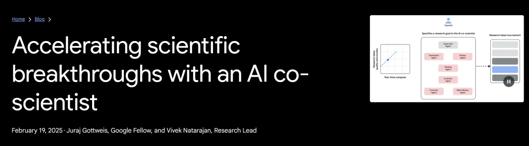
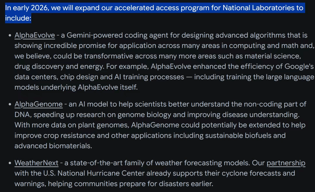
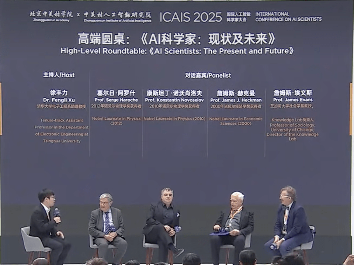
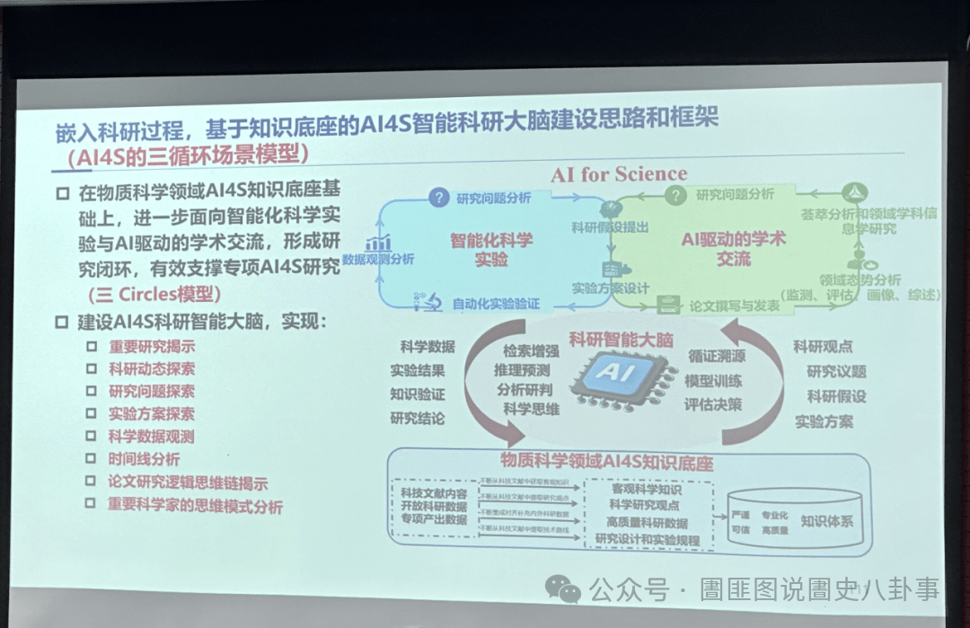
From isolated demos to national labs, frontier models, and closed-loop discovery platforms
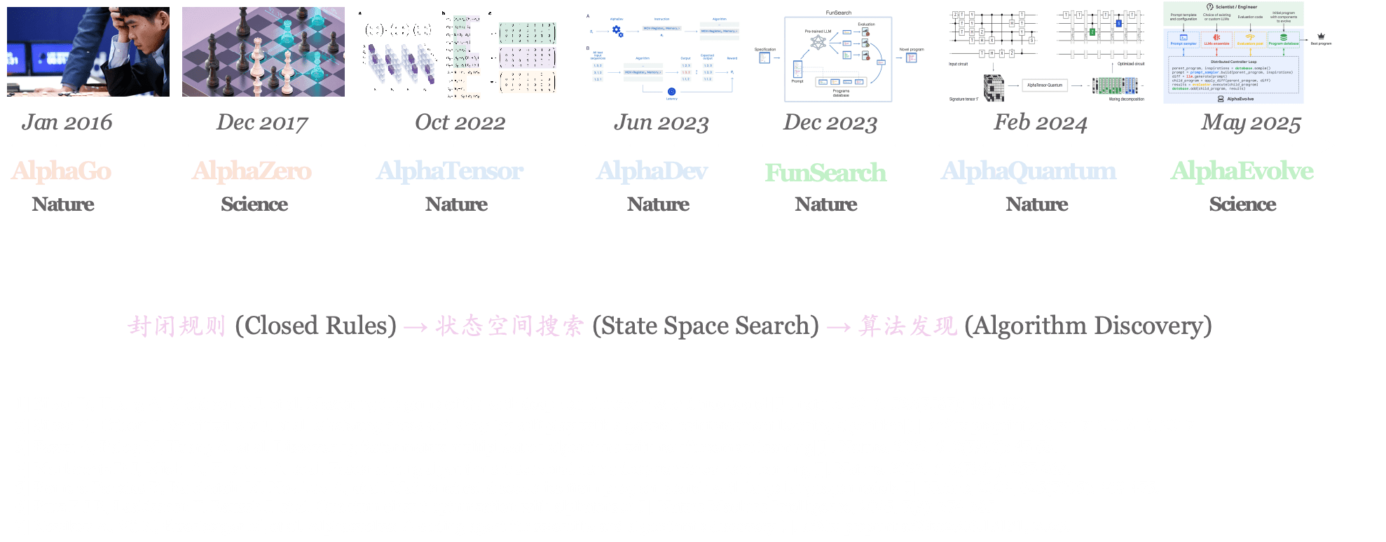
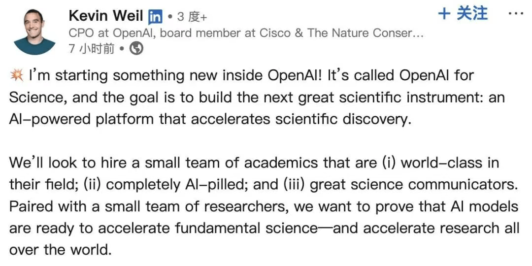
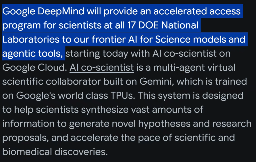
2025年的后半年,大家纷纷开始押注 AI for Science!
OpenAI 计划组建一个由顶尖学者组成的小型团队,这些学者需要满足三个条件:
这一系列举措表明,AI 驱动的科学发现正从学术探索迈向战略竞争新阶段。
# Discovery
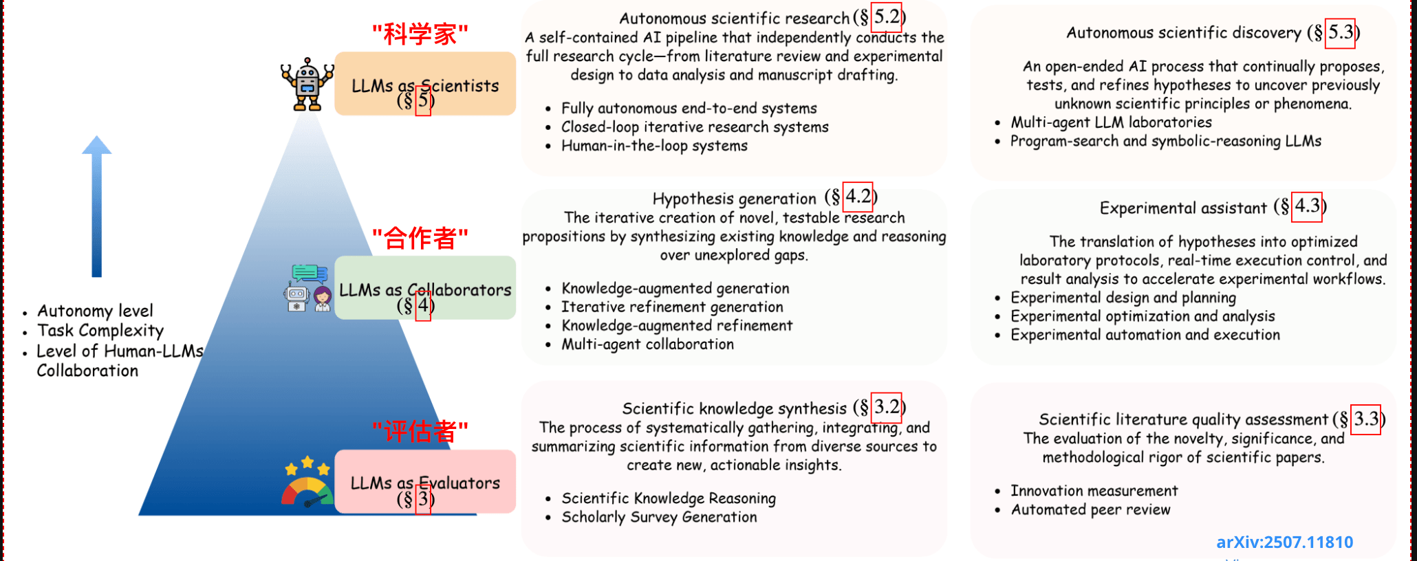
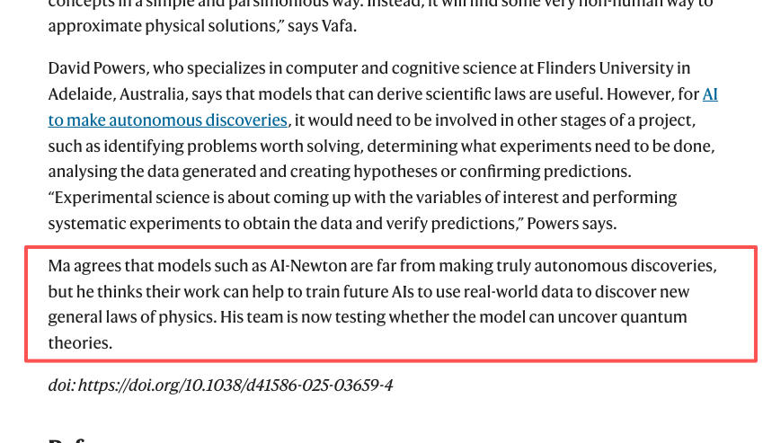
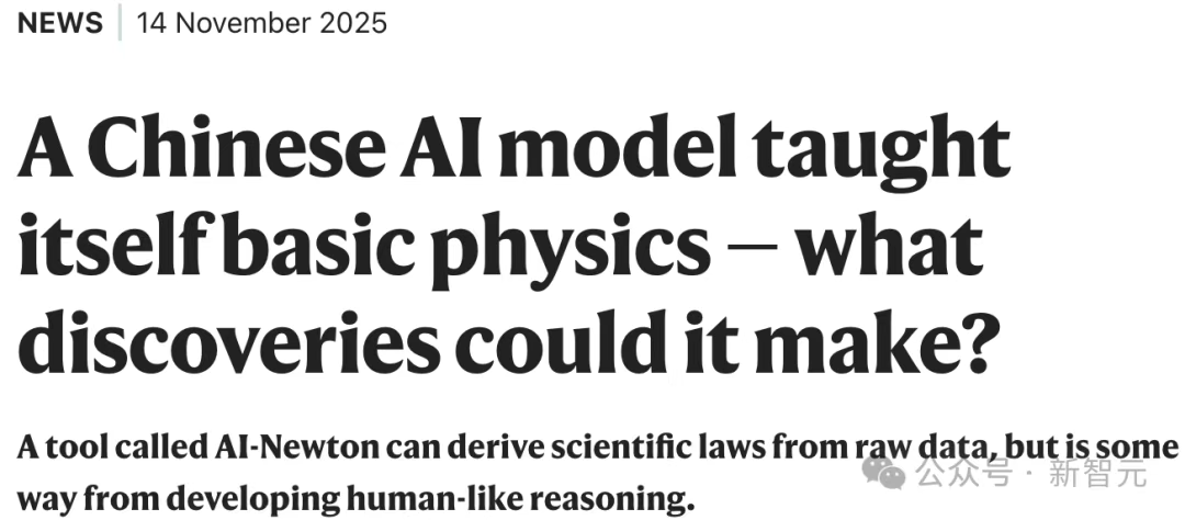
As autonomy increases, LLMs move from evaluating science to collaborating on it—and eventually conducting it.
# Discovery
Automation is progressing fast; scientific autonomy is not.
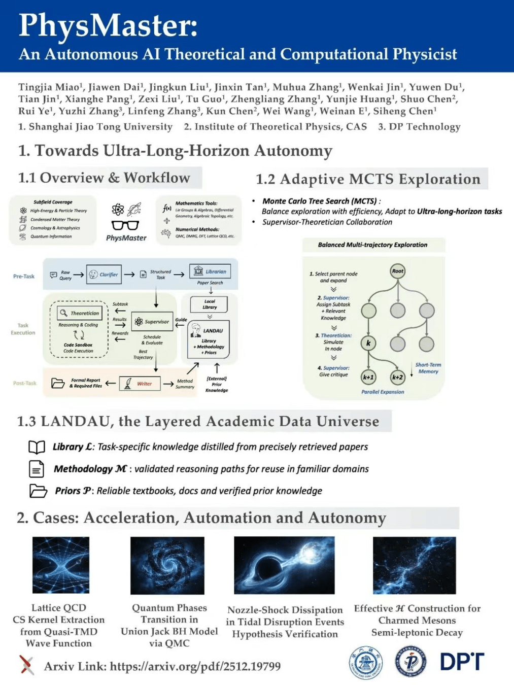
PhysMaster: 构建自主AI物理学家,面向理论与计算物理研究
arXiv:2512.19799 [cs.AI]
AI Scientist
AI Scientist 的天花板是什么?
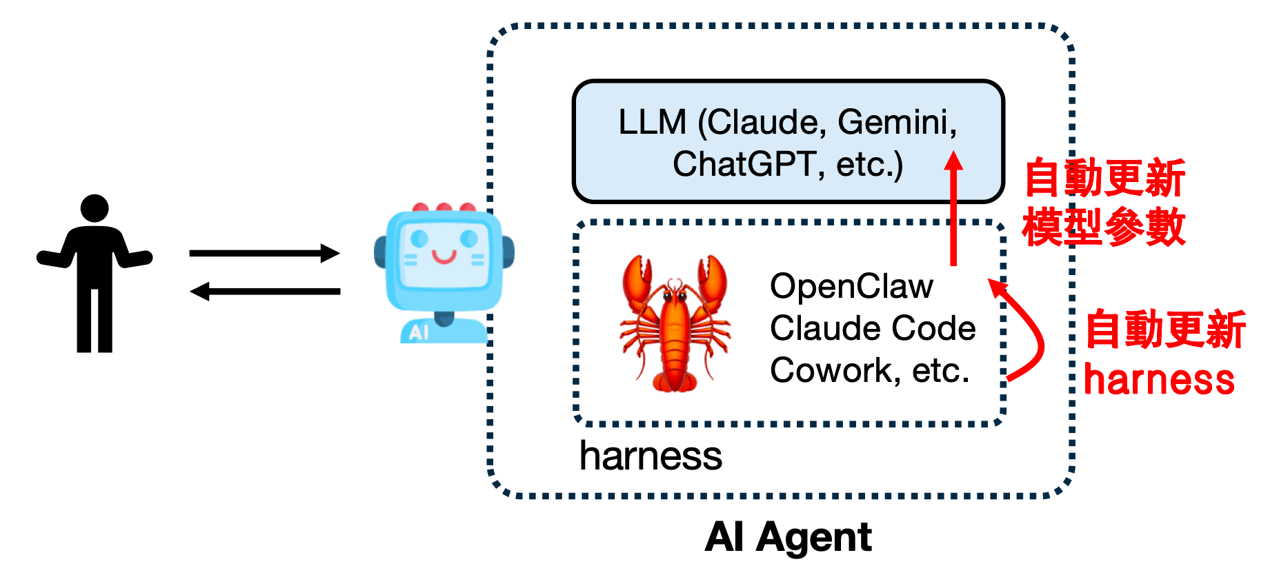
Understanding the Harness Behind Modern AI Agents
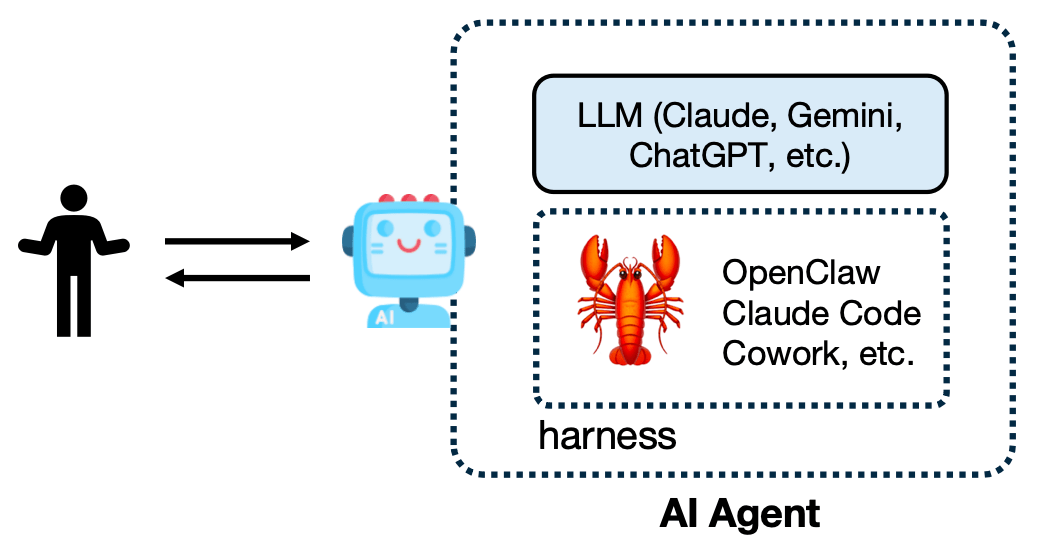
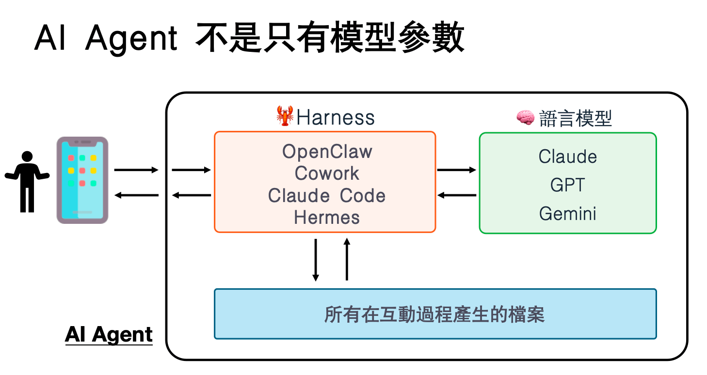
\(\boxed{\text{AI Agent}=\text{LLM}+\text{Harness}+\text{Environment}}\)
# Harness
What changes when the same LLM is placed inside a different harness?
你的任务是修复 `parser.py` 中的 bug。
目前 `extract_emails` 函数无法正确提取帶有 `-` 或 `_` 的 email 地址,例如 `test-user@domain.com`。
请修改 `parser.py`,使 `verify.py` 的测试能够完全通过。
You are an AI Agent. You can interact with the environment by writing code blocks.
If you write a ```bash\n...\n``` block, the system will execute it and return the output.
If you write a ```python\n...\n``` block, the system will execute it and return the output.
To finish the task, output 'DONE'.Provided tool;
沒有提供 “parser.py”
…… 我自己寫一個
parser.py
def extract_emails(text): ……
# Example test cases to verify the fix
test_string_1 = ……
DONE
# Harness
What changes when the same LLM is placed inside a different harness?
[CONTEXT]
You are running in a Linux environment (Google Colab). You need to find and modify the correct files to achieve the goal.

[INSTRUCTIONS]
1. Before modifying anything, you MUST inspect the current working directory, system environment, and file tree.
2. List all potentially relevant files.
3. Do not blindly modify files without looking at their contents first.


[DONE-WHEN]
You are done ONLY when the specific success criteria mentioned in the task are met, and the expected artifacts exist.
目前的环境
怎么工作
怎样算是完成
如果:增加一些额外的 prompt
# Harness
What changes when the same LLM is placed inside a different harness?
…
First, I will list the files.
```bash
ls -R
```
如果:增加一些额外的 prompt
--- Bash Execution ---
parser.py
verify.py
…
I will now display the content of `parser.py`.
```bash
cat parser.py
```--- Bash Execution ---
import re
def extract_emails(text):
……```bash
cat <<EOF > parser.py
def extract_emails(text):
……
EOF
```--- Bash Execution ---…
I will execute `verify.py`.
```bash
python verify.py
```--- Bash Execution ---
VERIFY_SUCCESS
如果:增加一些额外的 prompt
The model decides what to do; the harness decides how it works.
# Harness
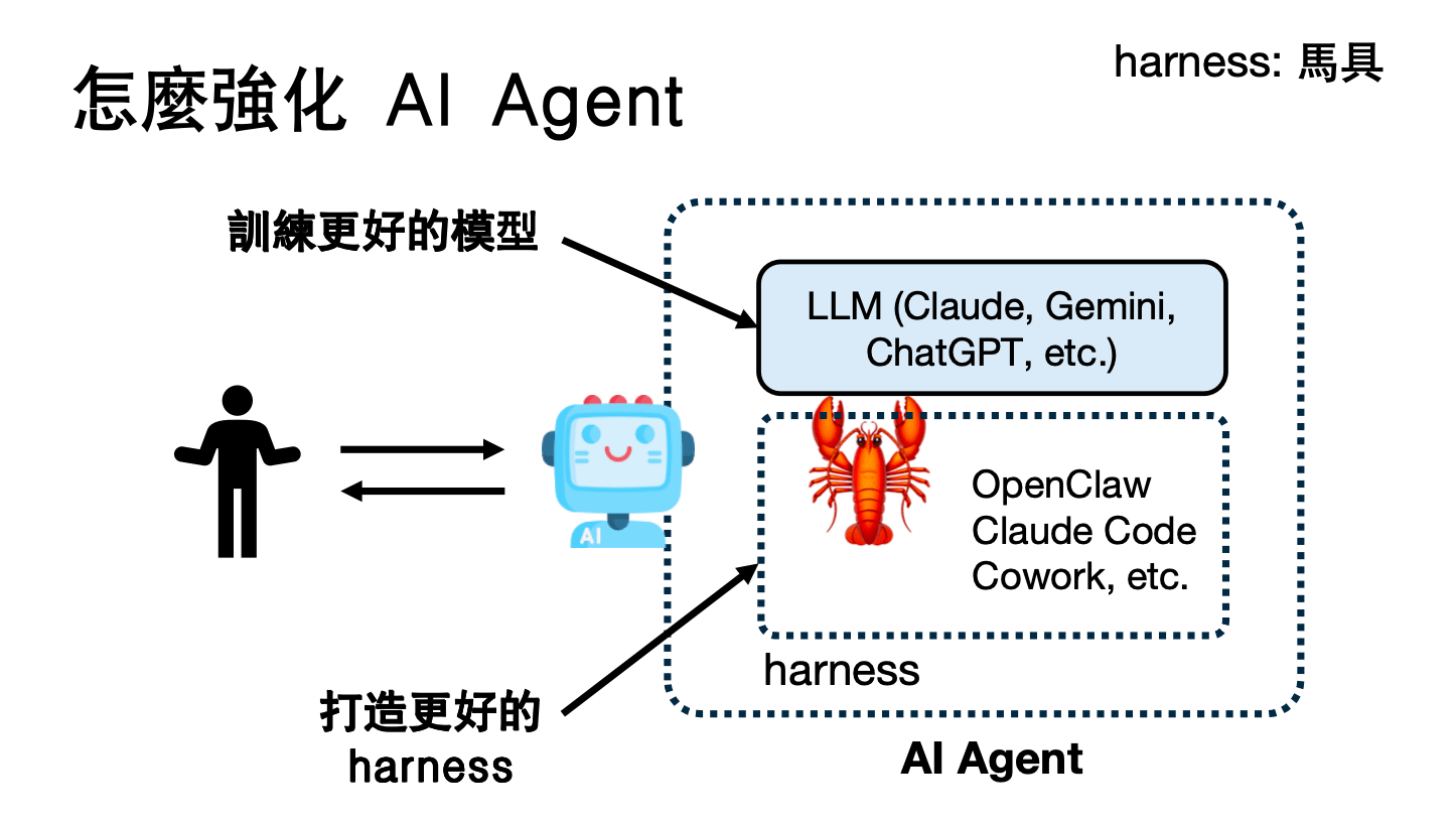
AI Agent 不是只有模型参数
训练更好的模型
打造更好的 Harness
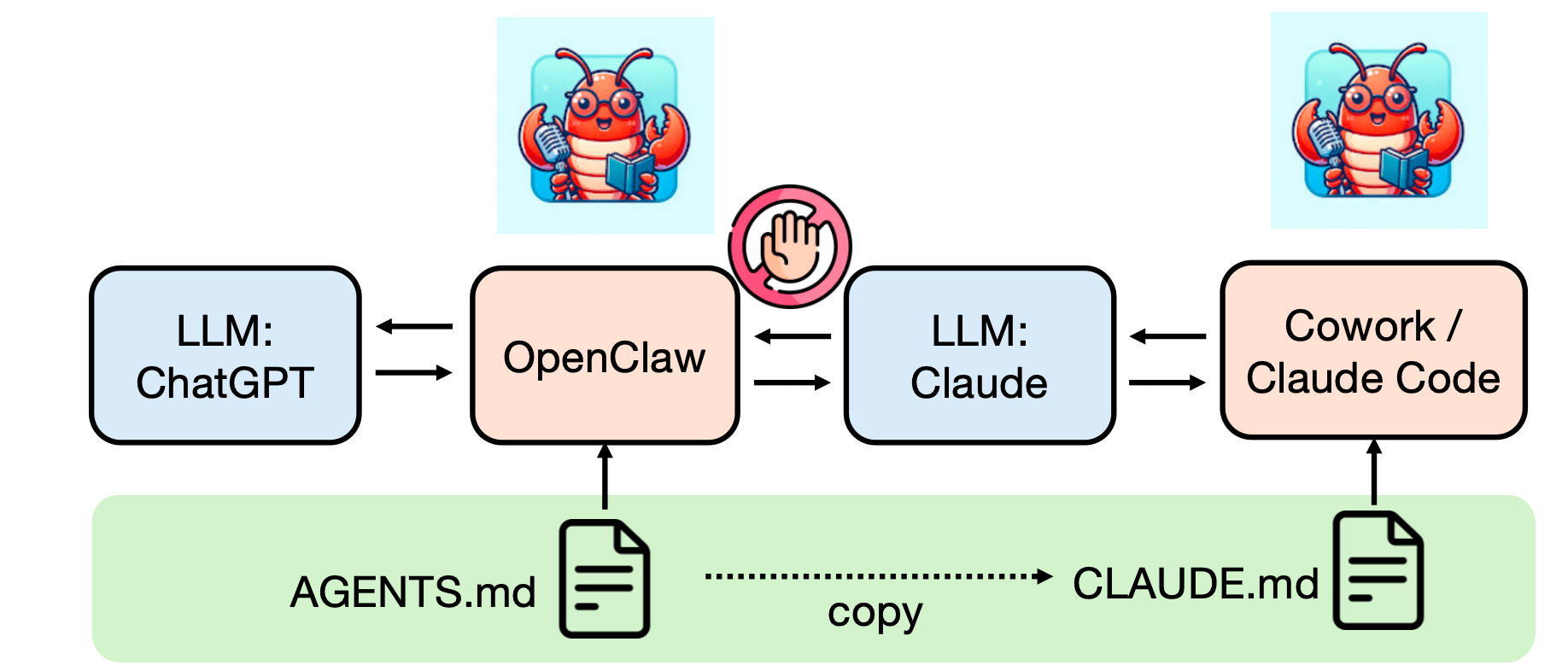
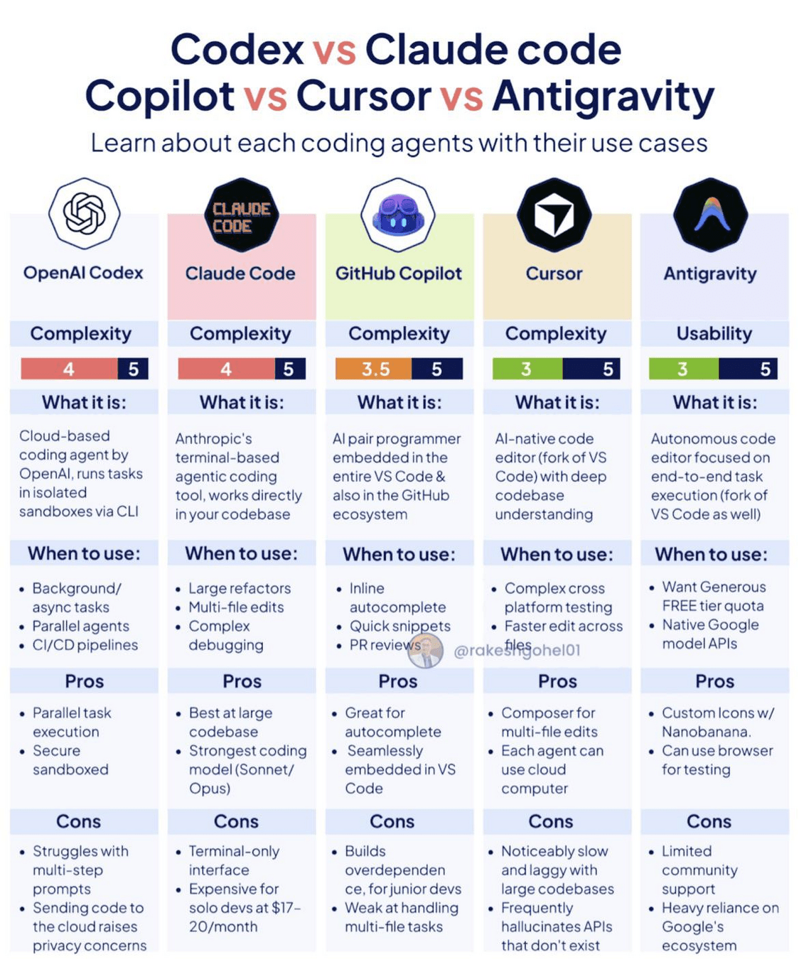
Claude Code、Codex CLI、OpenClaw……
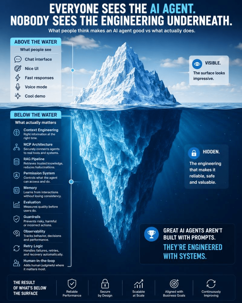
Much of today’s rapid progress comes from harness engineering, not only model scaling.
模型决定能力上限,Harness 决定能力能否真正发挥出来。
# Harness
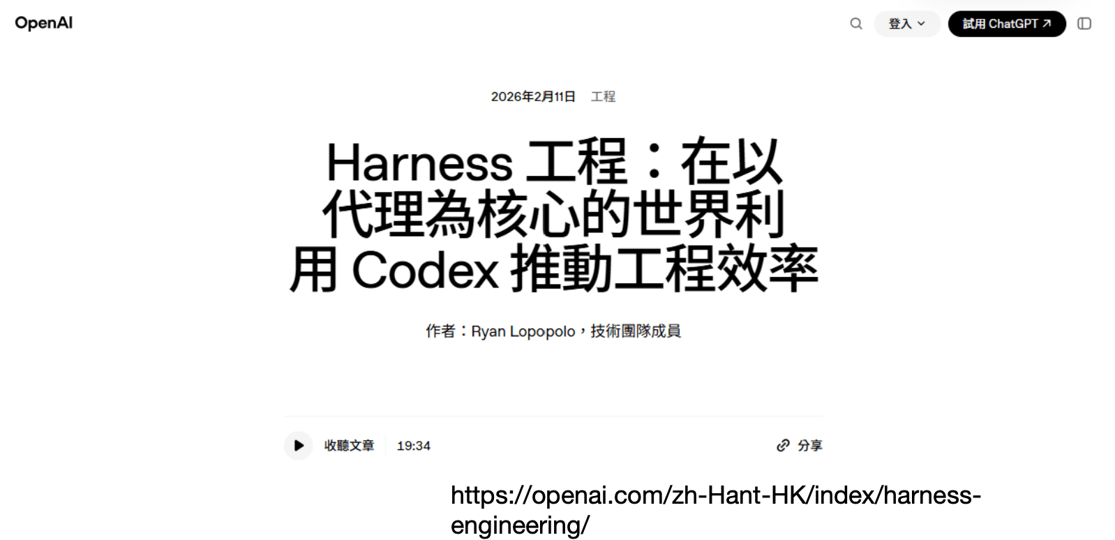
OpenAI officially introduces “Harness Engineering”.
The focus shifts from prompts to reliable systems.
Harness: equipment for controlling a horse
# Harness
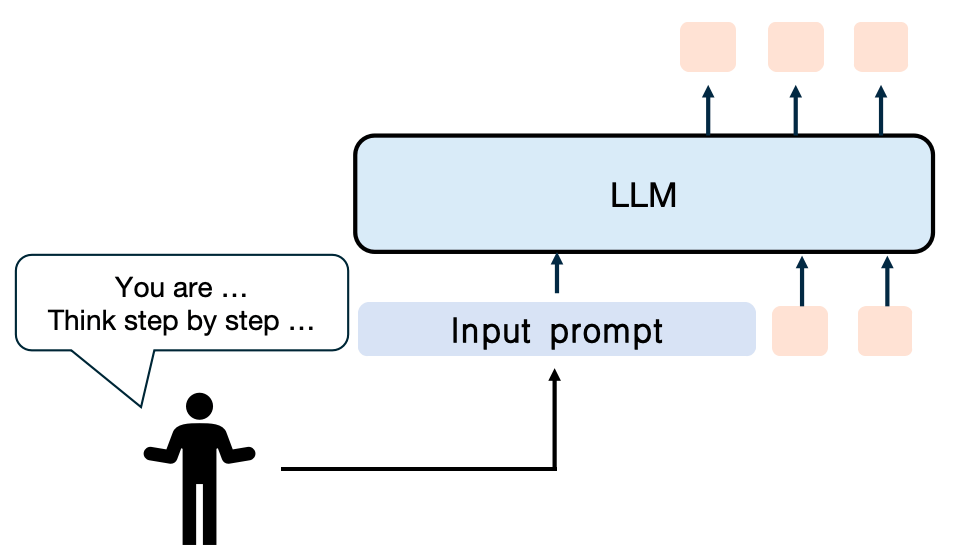
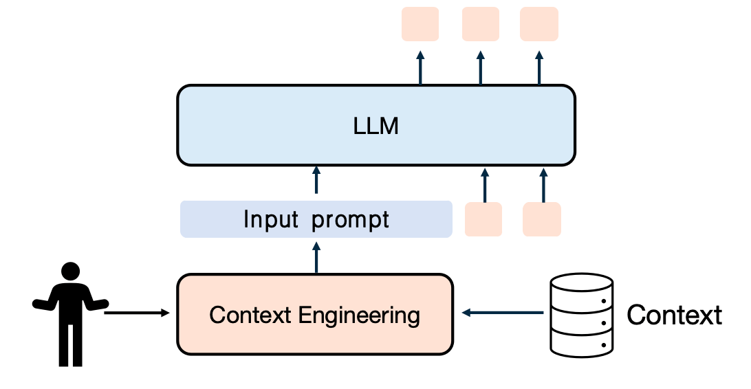
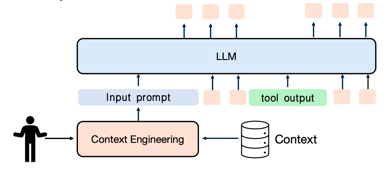
Engineering has shifted from prompts to systems.
Prompt Engineering(2023)
Everything is encoded into a single prompt.
Context Engineering(2024–2025)
Context, not the user, increasingly writes the prompt.
Harness Engineering(2025~)
The prompt becomes only one component of a complete execution system.
• Tool execution
• Context management
• Memory & State
• Planning & Reflection
• Verification & Recovery
# Harness
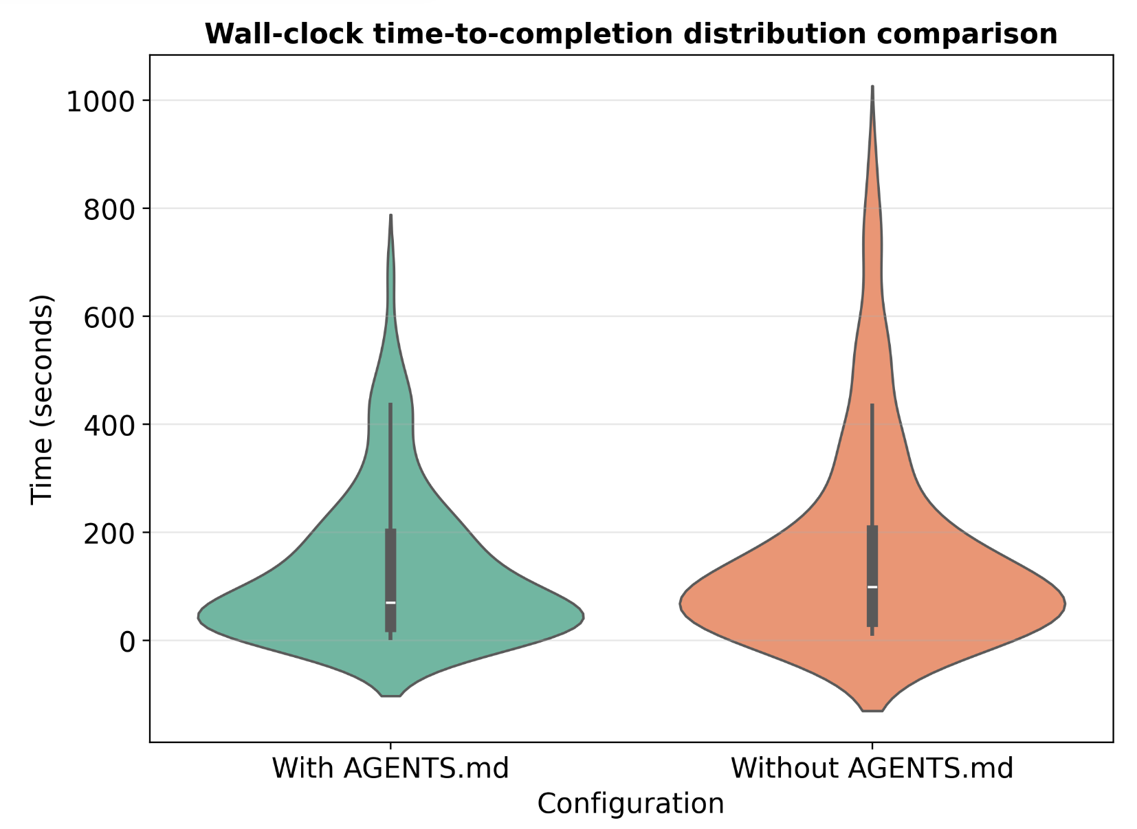
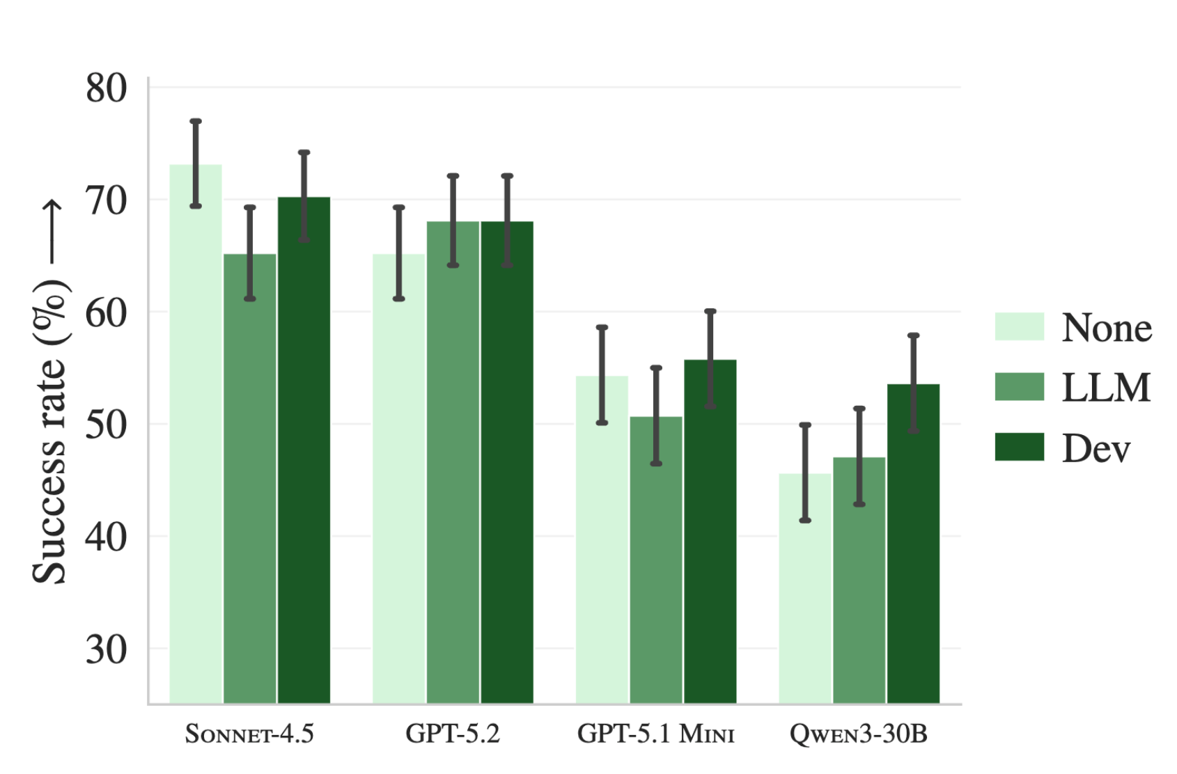
AGENTS.md and CLAUDE.md are examples of reusable harness specifications.
arXiv:2601.20404 [cs.SE]
arXiv:2602.11988 [cs.SE], https://agents.md/
Better harnesses complete tasks faster.
Better harnesses improve success rates.
# Harness
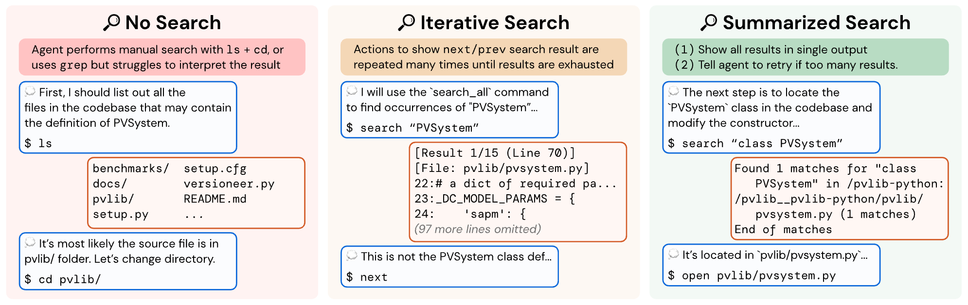
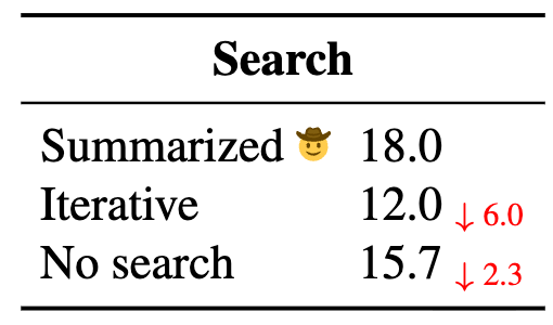
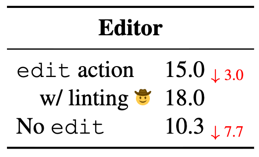
Better tools reduce reasoning and interaction overhead.
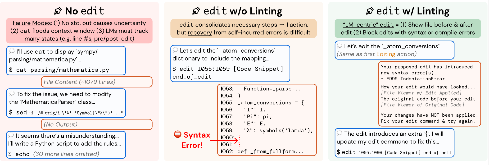
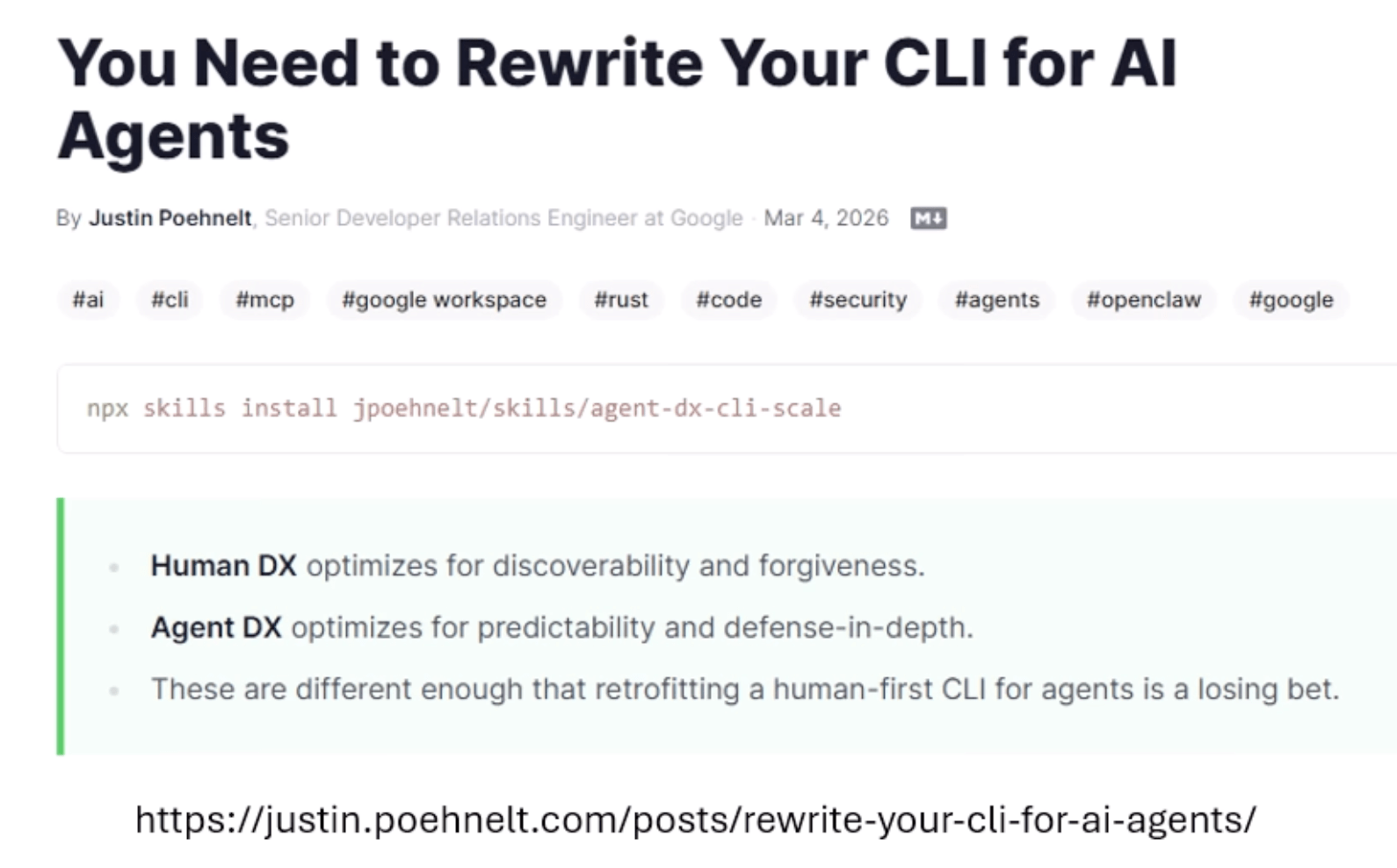
面向人类设计的工具,并不一定适合 AI Agent。
SWE‑agent (Agent-Computer Interface, ACI) (NeurIPS 2024)
# Harness
Better tools reduce reasoning and interaction overhead.
SWE‑agent (Agent-Computer Interface, ACI) (NeurIPS 2024)
面向人类设计的工具,并不一定适合 AI Agent。
# Harness
Better tools reduce reasoning and interaction overhead.
# Harness
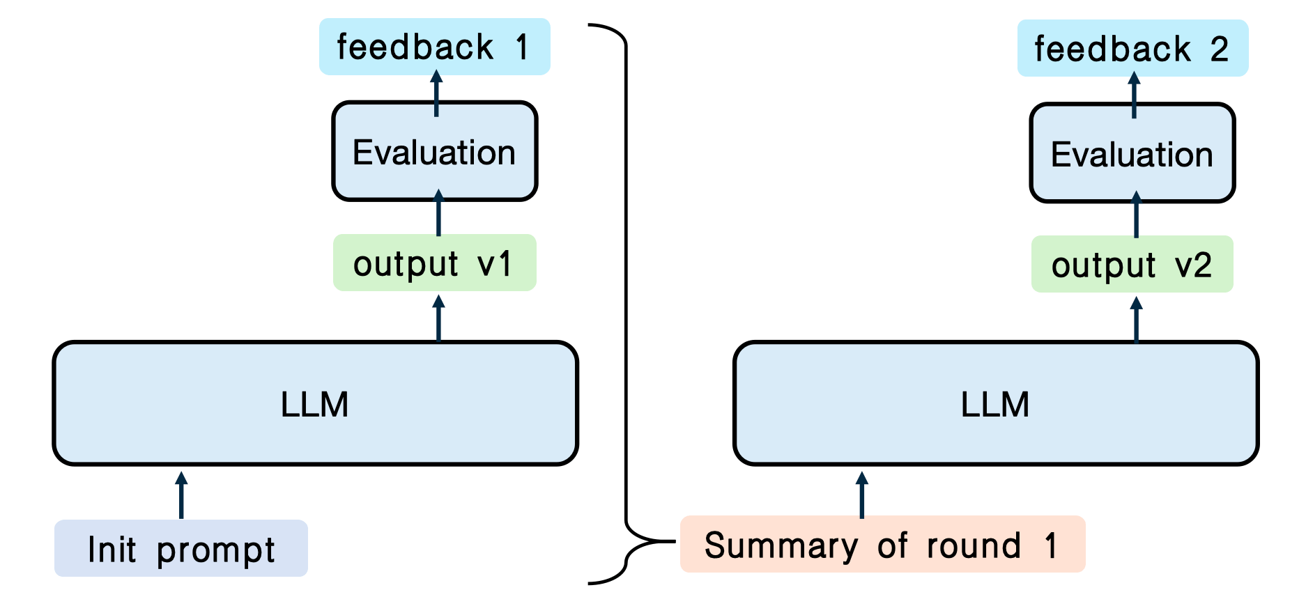
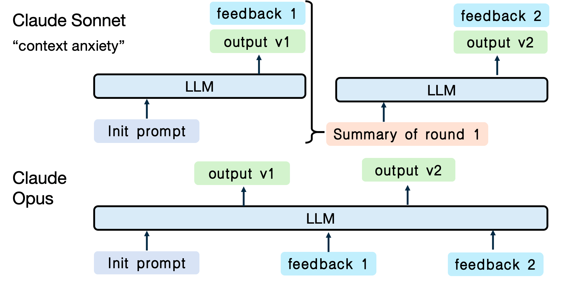
Long-running agents cannot simply keep appending history forever.
Context grows continuously.
Summaries replace raw interaction history.
https://ghuntley.com/ralph/
https://ghuntley.com/loop/
Recommended Reading
Ralph
— Standard workflow for AI coding agents
ghuntley.com/ralph
Loop
— Reliable agent execution loops
ghuntley.com/loop
# Harness
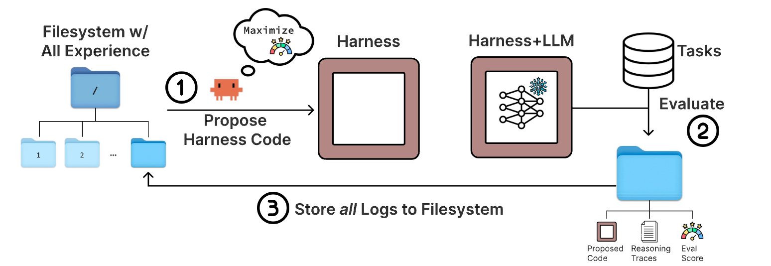
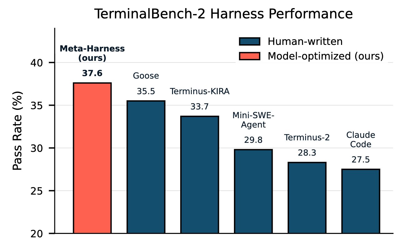
Beyond optimizing LLMs, we can optimize the harness itself.
Meta-Harness
arXiv:2603.28052 [cs.AI]
略
# Harness
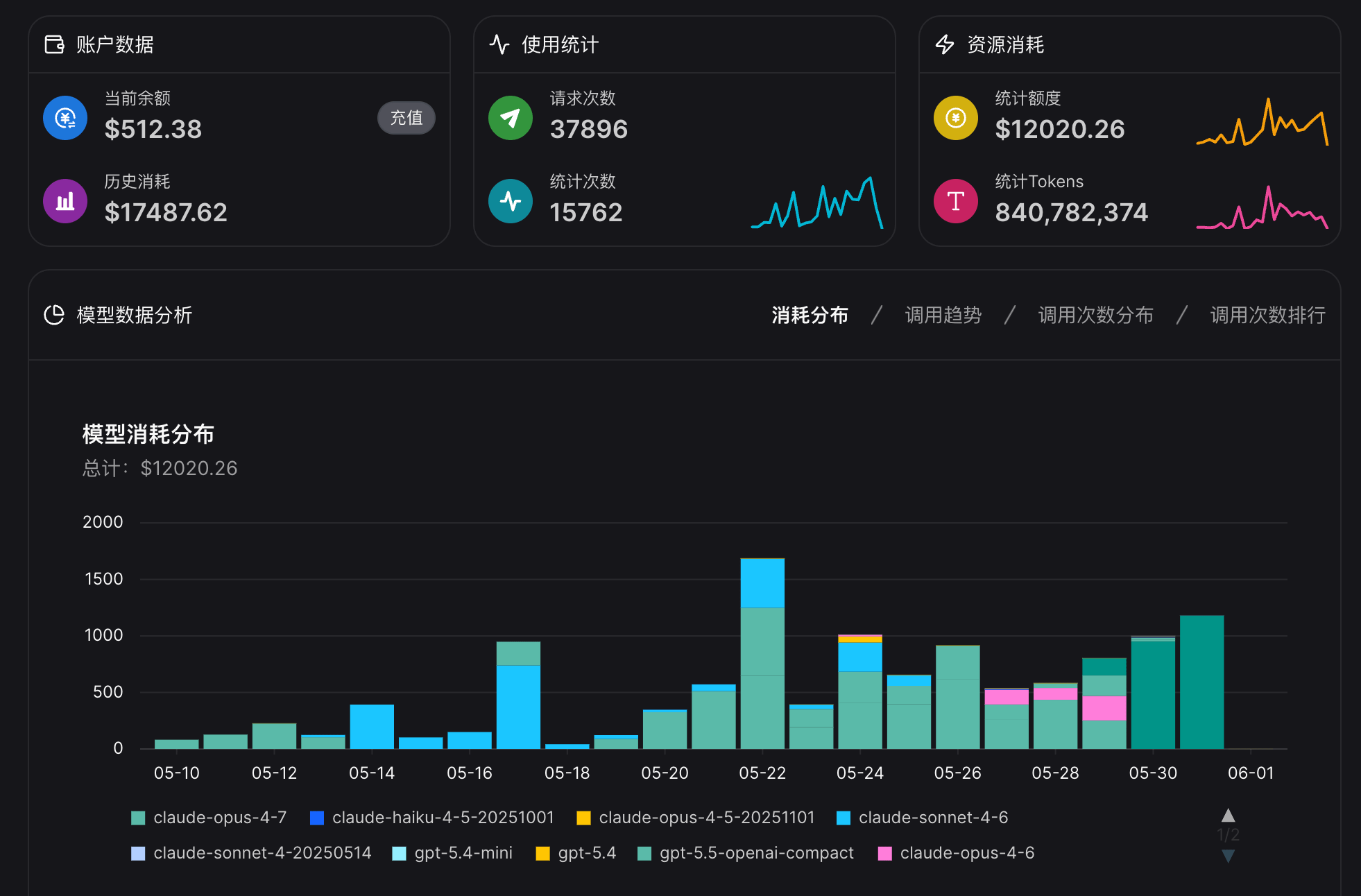
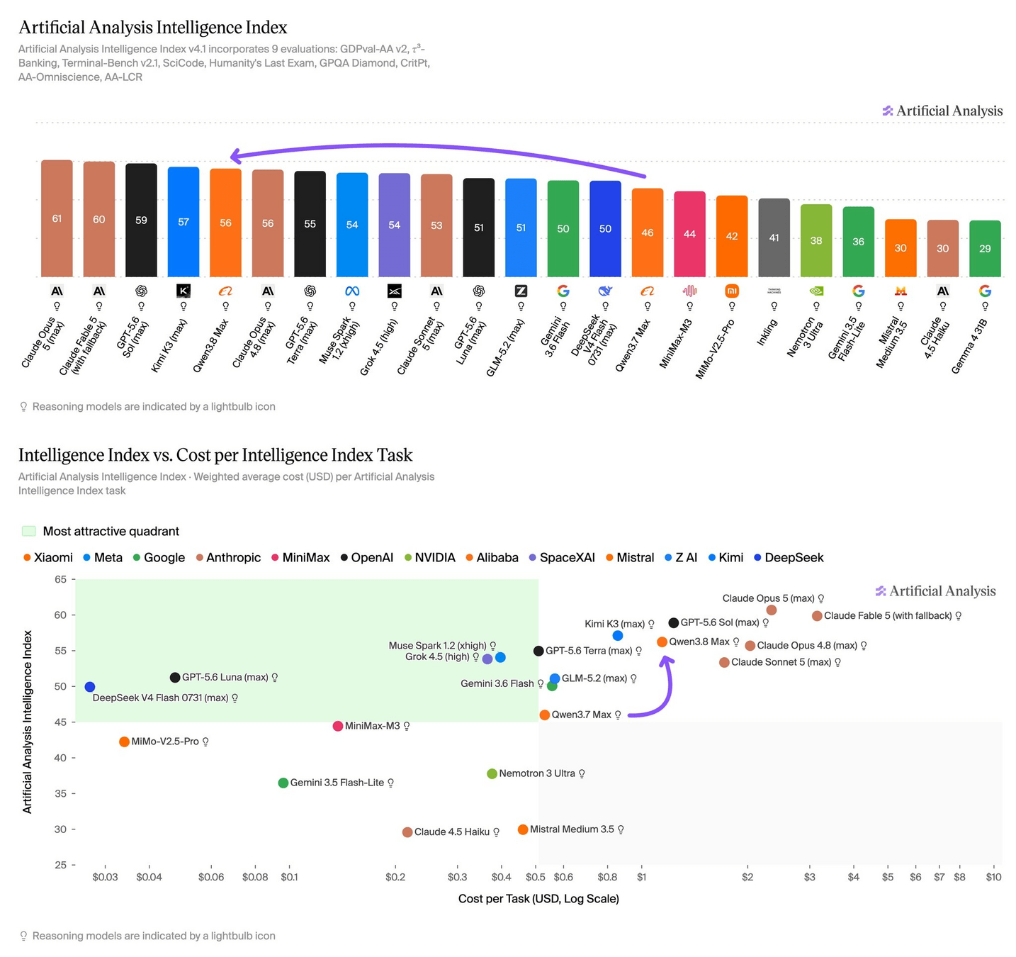
Choosing the right LLM and the right harness.
不要迷信只有一个”最好的模型”。
Switch models without changing workflows.
# Harness
Choosing the right LLM and the right harness.
# Harness
Choosing the right LLM and the right harness.
Navigating the Space of Ideas
# Harness
我想做一个实验。你可以随意问我任何一个问题,我会尽可能真实且完整地回答。基于我的回答,你再继续问下一个问题。我们会这样来回进行,持续下去,直到挖掘出我内心深处的构思——包括谬误、局限、潜能、需要改进的地方,或者任何潜藏在我潜意识中的东西。for _ in range(num_of_audiences):
print('Thank you for your attention! 🙏')太极实验室 2026 年度“大学生创新实践训练计划’
(引力波数据分析与 AI for Science 方向)
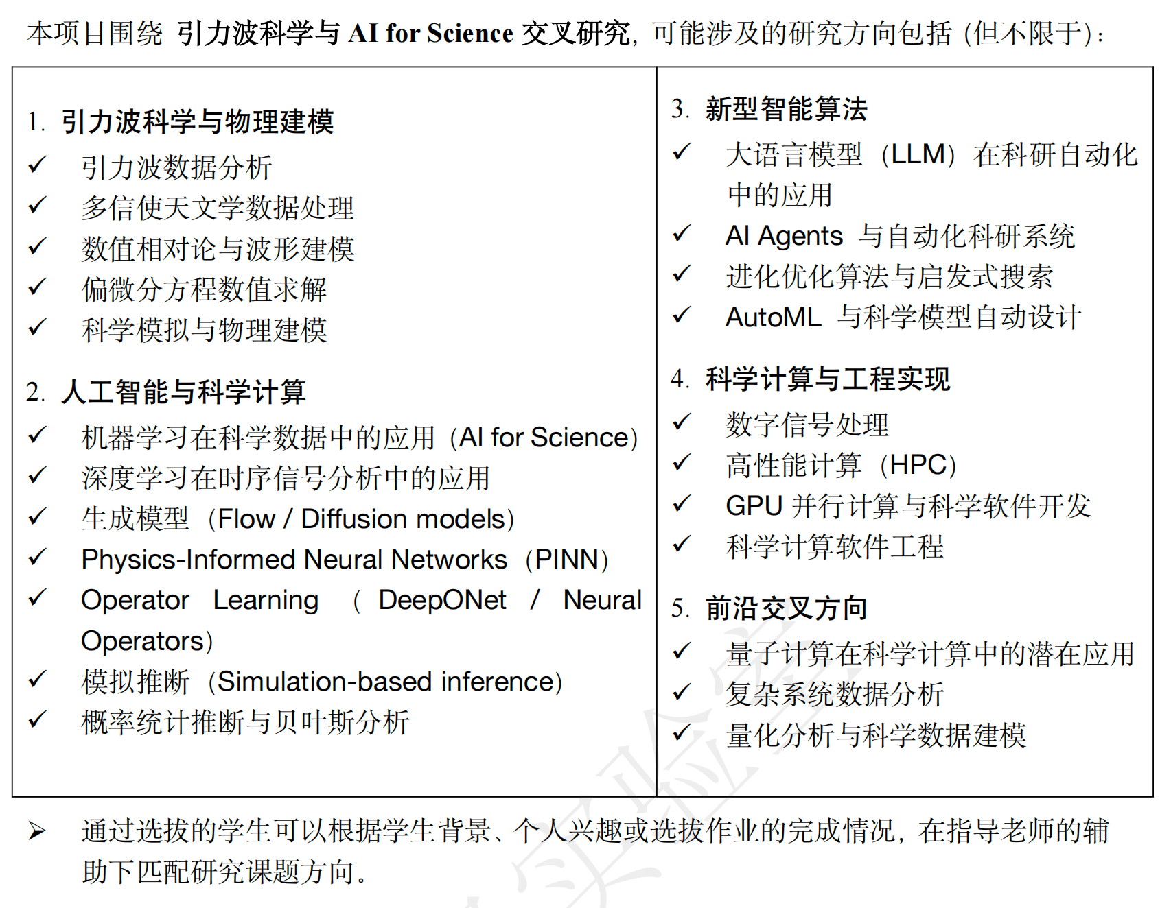
中国科学院大学引力波宇宙太极实验室(北京)引力波数据分析与机器学习课题组长期面向全国高校学生开放科研训练机会,现面向全国优秀学生招募参加太极实验室2026年度“大学生创新实践训练计划”,本课题组致力于探索引力波天文学、数值模拟与人工智能技术的交叉研究,重点发展新一代 Al for Science 方法,用于解决复杂物理系统建模、信号处理与科学数据分析问题,欢迎对 引力波科学、人工智能算法与科学计算 充满兴趣的同学加入,在真实科研项目中接受系统训练,并参与国际前沿研究。
https://github.com/iphysresearch/UndergradResearchLab/blob/main/2026科创计划及选拔题目.pdf
# End
By He Wang
2026 引力波数据分析暑期学校