










































![Delta_K^gzip,(d) = E[ CD(A1,B1) - 1/2 {CD(A1,A2) + CD(B1,B2)} ]](https://s3.amazonaws.com/media-p.slid.es/uploads/194679/images/13081291/image49.png)























Ishanu Chattopadhyay PRO
ML | Data Science Biomedical Informatics | Social Science | Assistant Professor
PI: Ishanu Chattopadhyay, PhD
Assistant Professor of Biomedical Informatics & Computer Science
University of Kentucky
DARPA-EA-25-02-05-MAGICS-PA-025
HR0011-26-3-E016
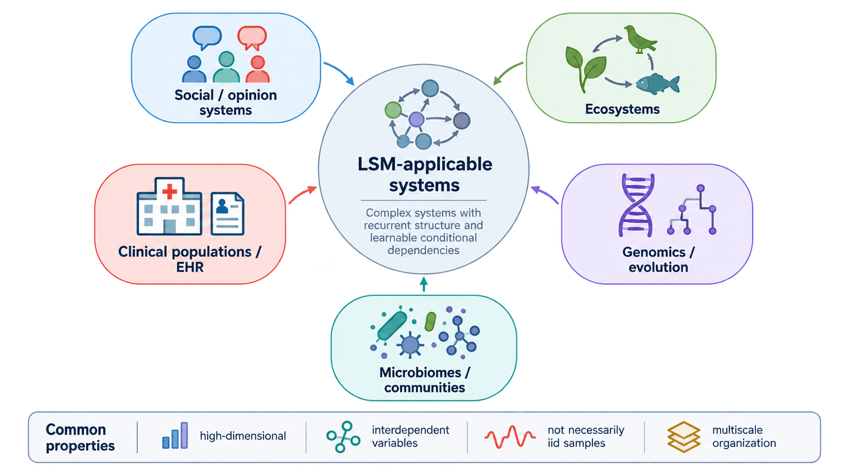
LSMs for complex systems arising in non-sequential multivariate measurements
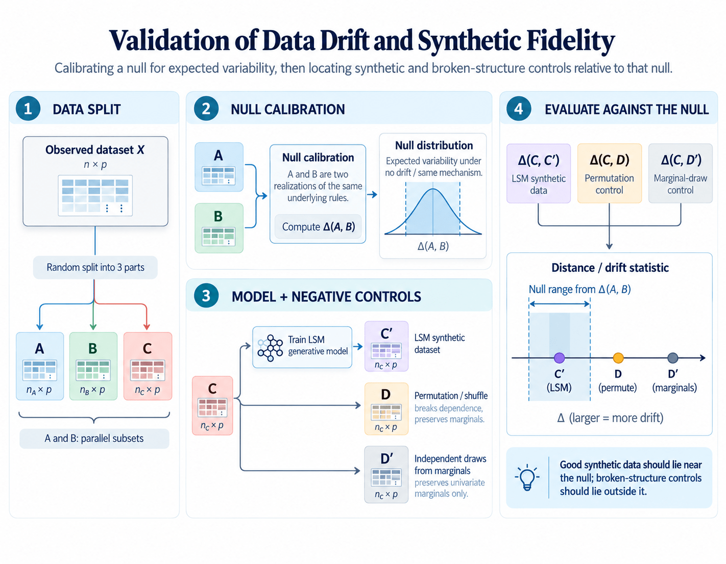
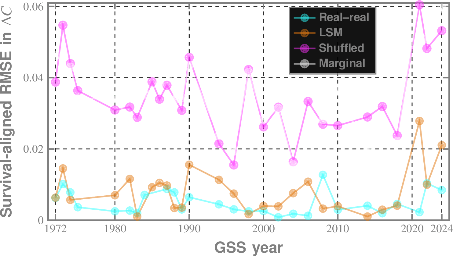
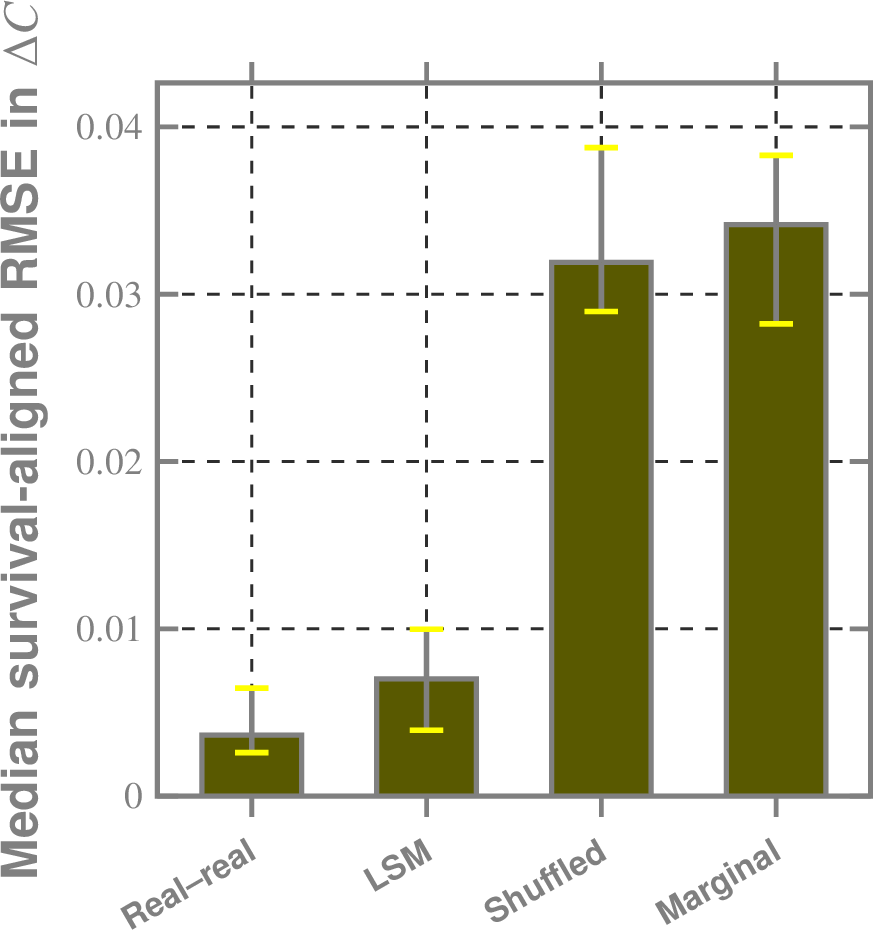
Validation?
At each depth \(d\), fit an LSM to the current population:
Score each observation by its conditional persistence:
Peel the low-persistence tail and refit:
Repeatedly isolate progressively less-persistent observations and relearn the conditional structure at every depth.
Normalized conditional support:
Conditional displacement:
Description length:
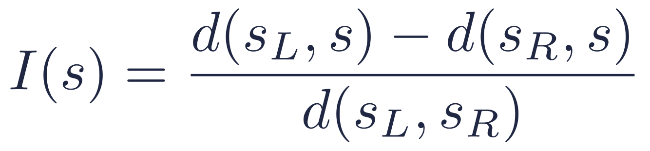
Information displacement:
multiscale spectrum is a data fingerprint
The trajectory across depth fingerprints how organization is distributed from persistent to progressively less-persistent structure.
“Exposure to opposing views on social media can increase political polarization” by Christopher A. Bail et al., published in PNAS in September 2018 (Vol. 115, No. 37, pp. 9216–9221; DOI: 10.1073/pnas.1804840115)
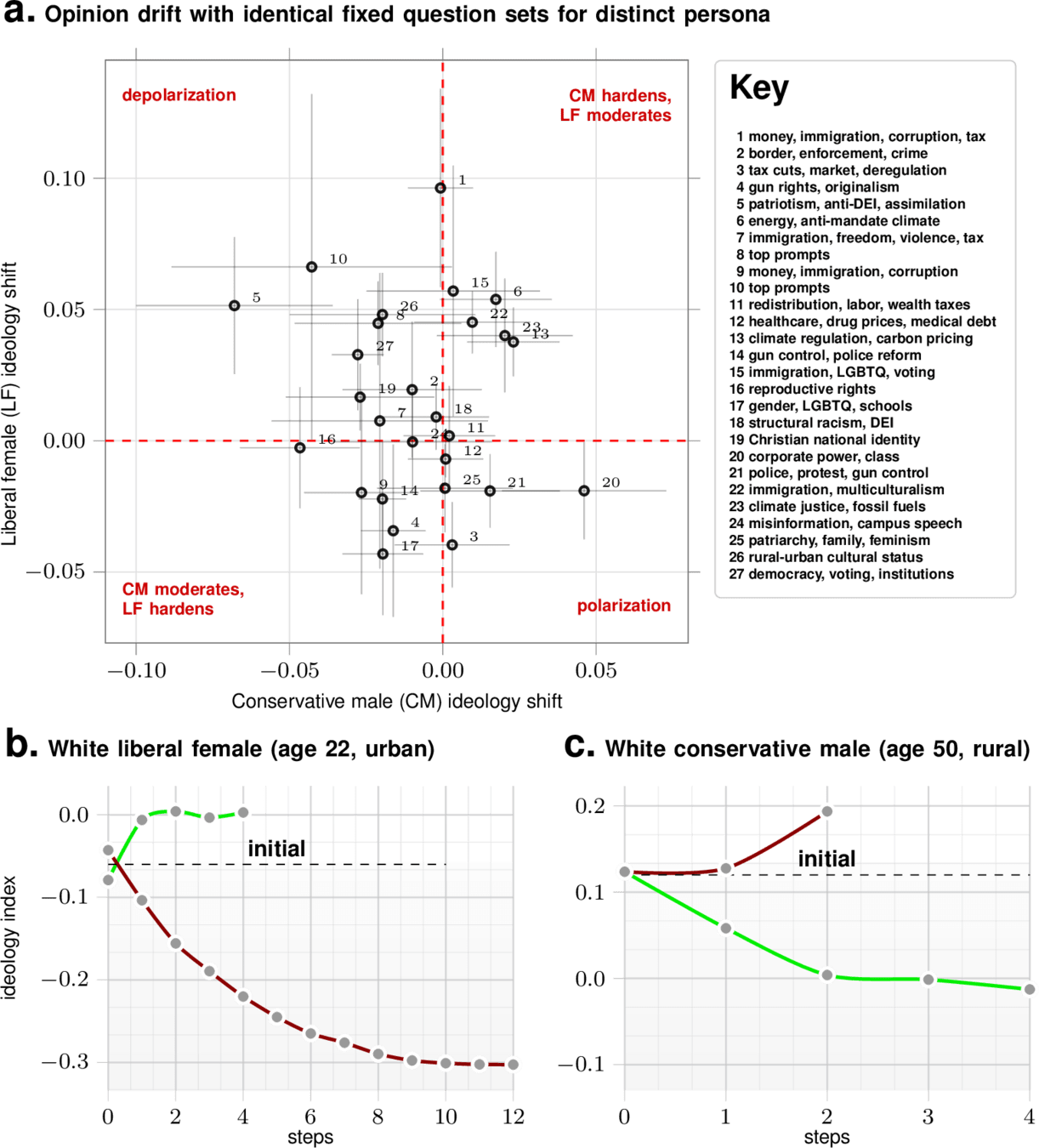
We find more general possibilities: We can make world-views go more extreme or less extreme based on the line of questions and the persona
Perturbing with opposing views made conservatives more conservative (statistically significant), liberals more liberal (not statistically significant)
LSM
Fixed Question Sets Exist That Move Different Persona Towards Polarization/Depolarization
We can optimize question sequences to move the same persona in a chosen direction
Note: It is relatively easy to polarize than to depolarize
SYSTEM-LEVEL DRIFT MEASUREMENT
The Characteristic Drift Spectrum
A task-free, multiscale fingerprint of systemic organization in complex systems
Systemic drift, not just more data from the same system.
Structural drift
Information drift
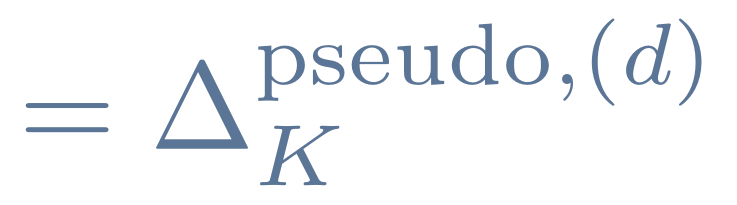
Kolmogorov drift
Ishanu Chattopadhyay
University of Kentucky
THE PROBLEM
More data is not drift
Characteristic Drift Spectra of Complex Systems
2 / 18
Two samples from an unchanged system never match row for row. A drift measure must ignore this re-realization noise and respond when the system’s organization changes.
Illustrative example: two survey items A and B, n = 1,000 per sample
SYSTEM P · SAMPLE 1
same organization
B yes
B no
A yes
396
104
A no
97
403
Yes-rates of A, B: 0.500, 0.493
P(B = yes | A = yes / no)
0.792 / 0.194
SYSTEM P · SAMPLE 2
same organization, new draw
B yes
B no
A yes
412
93
A no
104
391
Yes-rates of A, B: 0.505, 0.516
P(B = yes | A = yes / no)
0.816 / 0.210
SYSTEM Q · SAMPLE
items decouple; yes-rates unchanged
B yes
B no
A yes
247
254
A no
251
248
Yes-rates of A, B: 0.501, 0.498
P(B = yes | A = yes / no)
0.493 / 0.503
Marginal checks: the resample shifts more (up to 0.023) than the reorganized system (at most 0.005).
Conditional relation: 0.79 → 0.82 on resampling, but 0.79 → 0.49 when the items decouple.
Drift should mean the system changed, not that we drew new data.
WHAT DRIFT SHOULD MEAN
Re-realization or reorganization?
Characteristic Drift Spectra of Complex Systems
3 / 18
We want a drift measure that is a property of the system, not of the particular sample: its estimate should settle as data accumulate, and move only when the organization moves.
SAME ORGANIZATION P
Re-realization
Independent samples differ only as realizations. With stable, consistent conditional learning and estimation:
CHANGED ORGANIZATION P → Q
Reorganization
If the change alters the conditional organization, the residual hierarchy, or the information structure the probes interrogate, then S(P) and S(Q) need not coincide. The displacement persists rather than vanishing as a finite-sample effect.
Distance between estimated spectra
same organization: → 0
changed: persists
sample size n, m
schematic
Repeated realizations of the same organization approach the same fingerprint; organizational drift deforms that fingerprint.
CONDITIONAL ORGANIZATION
Learning the conditional organization
Characteristic Drift Spectra of Complex Systems
5 / 18
For categorical state X = (X1, …, Xp) and row population R, a conditional learner returns target-wise predictors φi of Xi given X−i:
For row x, the mean conditional log-persistence is
PM(x) is the average log support assigned to the observed coordinates when each coordinate is predicted from the remainder of the state.
Low persistence identifies rows that are poorly reconstructed by the dominant learned conditional organization.
Learner-agnostic. The objective is the full family of conditionals, not one selected response. Any sufficiently accurate and stable conditional learner can instantiate the spectrum; the GSS results use Large Science Models (LSMs) [5, 6].
Masked-coordinate prediction
x1
x2
x3
?
masked
⋯
xp
MAP
observed
Conditional distribution over states a ∈ Ai
INTRINSIC RESIDUAL HIERARCHY
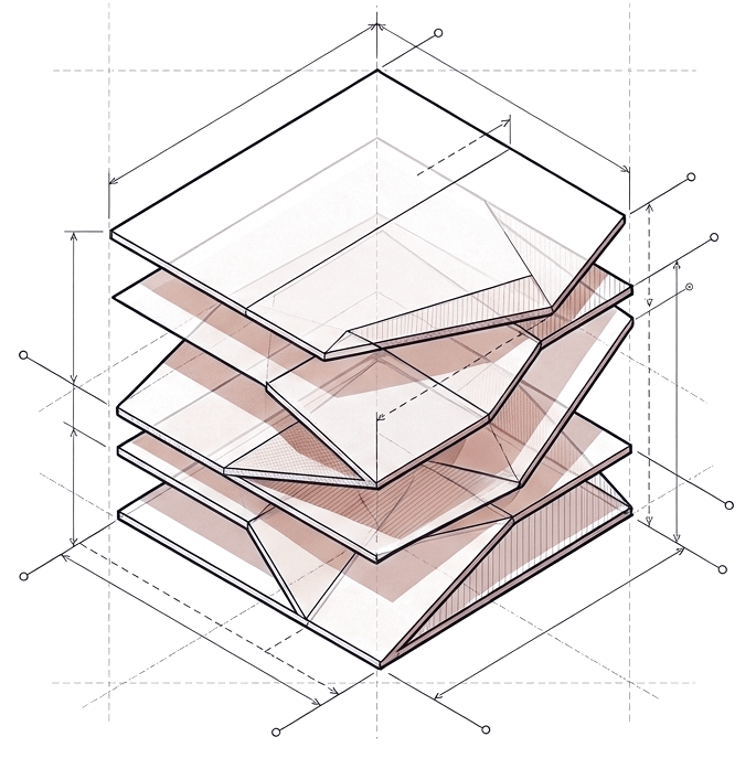
Peeling recovers a residual hierarchy
Characteristic Drift Spectra of Complex Systems
6 / 18
⋮
a freshly fitted conditional model at every level
1
Fit and score
2
Robustly standardize lack of persistence
3
Peel and refit
At depth d, fit a conditional model Md = M(Rd) and compute the persistence of every row under Md.
Intuition. Peeling removes the statistically dominant core and refits on the surviving low-persistence population, so organization masked at the population level becomes visible. Depth is structural, not chronological.
COORDINATES OF THE SPECTRUM
Three nonredundant probes at every depth
Characteristic Drift Spectra of Complex Systems
7 / 18
PROBE I
Structural drift
ASKS
Does MAP-normalized reconstruction change after refitting?
SENSITIVE TO
Reconstruction geometry
PROBE II
Information drift
ASKS
Does the residual population have a different conditional description length under the parent organization?
SENSITIVE TO
Conditional description length
PROBE III
Kolmogorov drift
ASKS
Are adjacent residual populations distinguishable through compression, without the fitted model as the measuring instrument?
SENSITIVE TO
Model-independent compressibility
Why three? The probes need not move together: information drift can be nonzero even when structural drift is zero. Collapsing them to one coordinate would discard distinguishable forms of reorganization.
PROBE I
Structural drift
Characteristic Drift Spectra of Complex Systems
8 / 18
MAP-normalized masked-state reconstruction score
uM = 1 when the observed state attains the conditional MAP support; smaller values measure its support relative to that MAP state.
With a balanced probe cloud Qd and common evaluable targets Id(x), average the change between adjacent depths:
Same probe, adjacent depths
MAP state
observed state
Intuition. Structural drift measures how the system’s learned ability to reconstruct masked coordinates changes across structural depth.
PROBE II
Information drift
Characteristic Drift Spectra of Complex Systems
9 / 18
A data-adaptive code from the learned conditional structure
Mean code length (bits) of row x when each coordinate is encoded with the fitted conditional predictor.
Information drift between adjacent residual levels
Both expectations use the parent model Md: rows of Rd+1 are coded under the organization learned on Rd.
Mean code length under Md
schematic
Intuition. A conditional-model-based description-length probe: information displacement is measured using structure learned from the system itself.
PROBE III
Kolmogorov drift
Characteristic Drift Spectra of Complex Systems
10 / 18
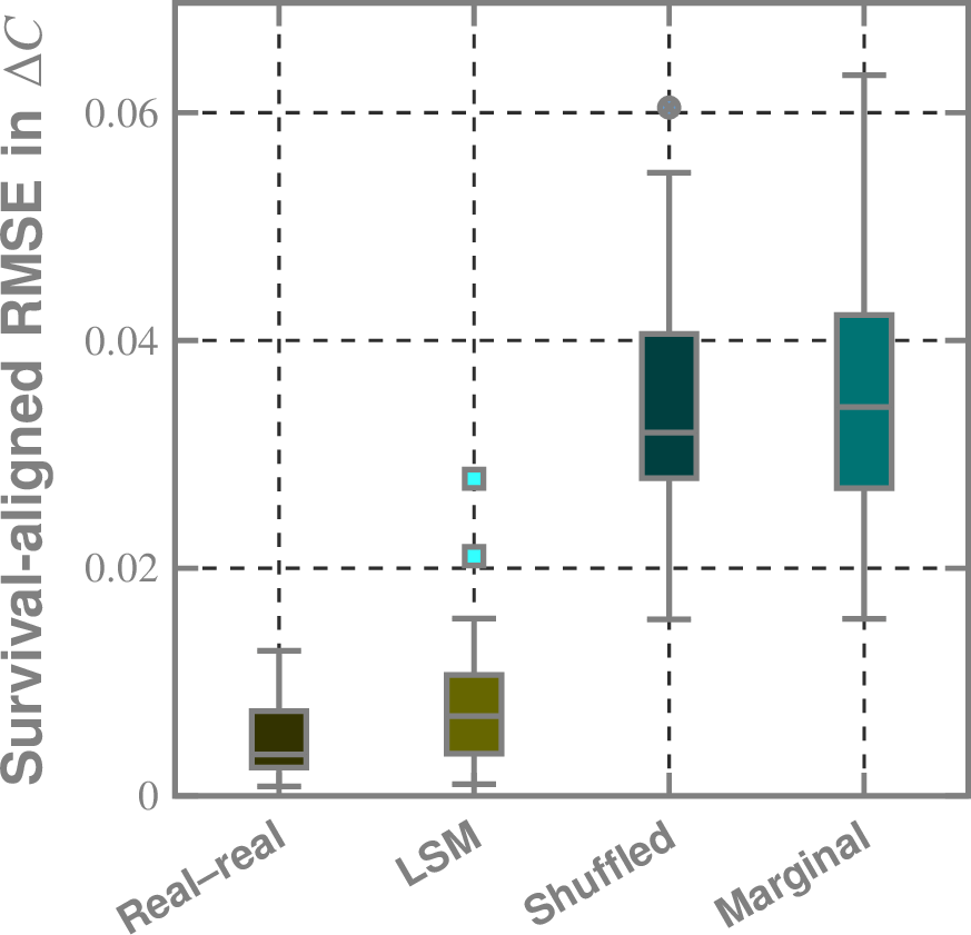
At depth d, draw matched row blocks A1, A2 ⊂ Rd and B1, B2 ⊂ Rd+1. For serialized blocks a, b and compressor length C(·), the normalized compression distance is
Within-depth distances establish the intrinsic compression scale; the across-depth distance measures separation between adjacent levels:
within depth: intrinsic scale
across depth: separation
Intuition. Compression-calibrated information displacement between adjacent residual levels, without using the fitted conditional model as the measuring instrument.
POSITIVE CONTROL
GSS: recovering a known data shift
Characteristic Drift Spectra of Complex Systems
12 / 18
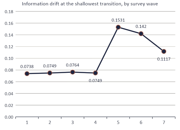
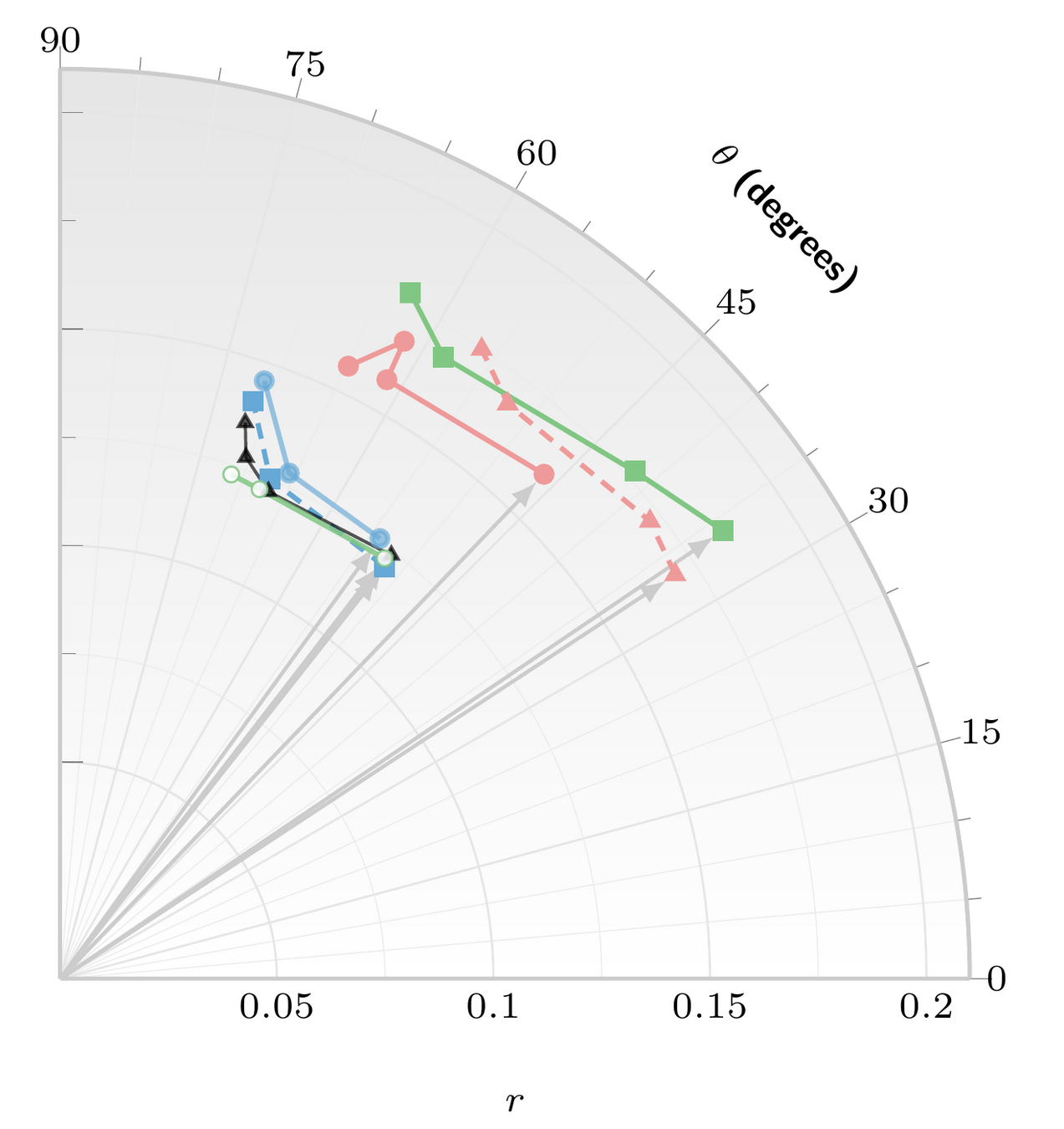
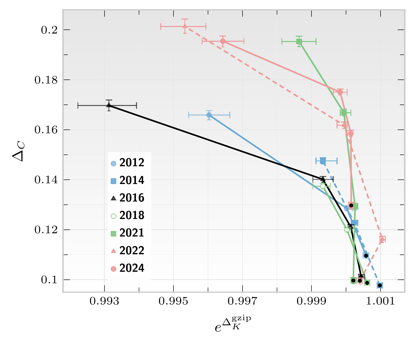
0.0738–0.0764
2012–2018 · four waves, one design
Re-realization: nearly the same value
0.1531
2021 · primarily web-based
Shift ≈ 30× the 2012–2018 spread
0.1420 → 0.1117
2022, 2024 · mixed web/face-to-face
Partial return toward the earlier regime
Conditionals estimated with our LSM implementation, one instantiation of the conditional-learning objective rather than a requirement of the spectrum.
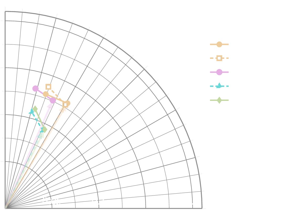
Repeated waves under one design give nearly the same fingerprint; the documented design change displaces it, without training to discriminate years or modes.
SYNTHESIS
The characteristic drift spectrum
Characteristic Drift Spectra of Complex Systems
11 / 18
At every depth d, the three numbers form
and stacking them across depth gives a depth-by-coordinate matrix:
⋮
⋮
⋮
rows: structural depth d = 0, …, D−1 columns: the three probes
A task-free, multiscale fingerprint: repeated realizations of the same organization approach the same matrix, persistent displacement signals reorganization, and depth localizes where it occurs.
POSITIVE CONTROL
Two projections of the GSS spectrum
Characteristic Drift Spectra of Complex Systems
13 / 18
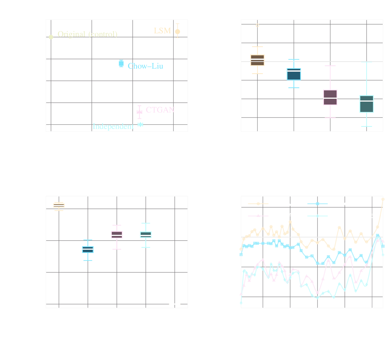
a Polar rendering of the raw (information drift, structural drift) plane. A tight 2012–2018 regime, a pronounced 2021 displacement, and partial return in 2022 and 2024.
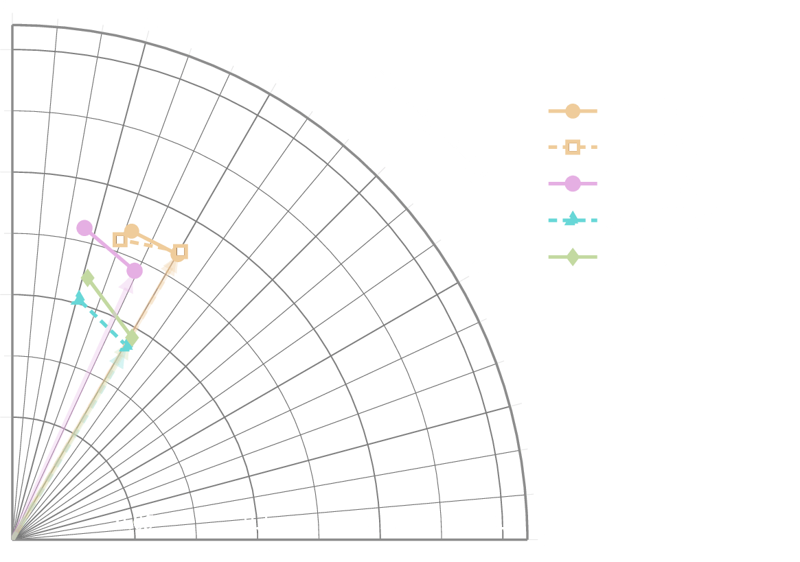
b gzip/NCD information displacement against the Dirichlet-posterior mean of structural drift; the horizontal axis shows exp(Kolmogorov drift).
MULTISCALE COMPARISON
Spectra as fingerprints: 2018 vs 2024
Characteristic Drift Spectra of Complex Systems
14 / 18
d = 0
.0971
.0749
.00061
d = 1
.1130
.0460
.00004
d = 2
.1164
.0395
−.00090
d = 0
.1165
.1117
.00015
d = 1
.1383
.0754
−.00008
d = 2
.1472
.0794
−.00035
First three transitions; cell shading scales with value within each of the first two columns.
Reading the fingerprints
Shallowest transition: information drift rises from .0749 (2018) to .1117 (2024).
2024 exceeds 2018 in both structural and information drift at all three depths.
Structural drift grows with depth in both years; Kolmogorov drift stays below 0.001 in magnitude.
Repeated observations can be compared through their full spectra rather than a single classifier or one global distance.
SECOND SURVEY PROGRAM
Eurobarometer: ten waves, 2018–2021
Characteristic Drift Spectra of Complex Systems
15 / 18
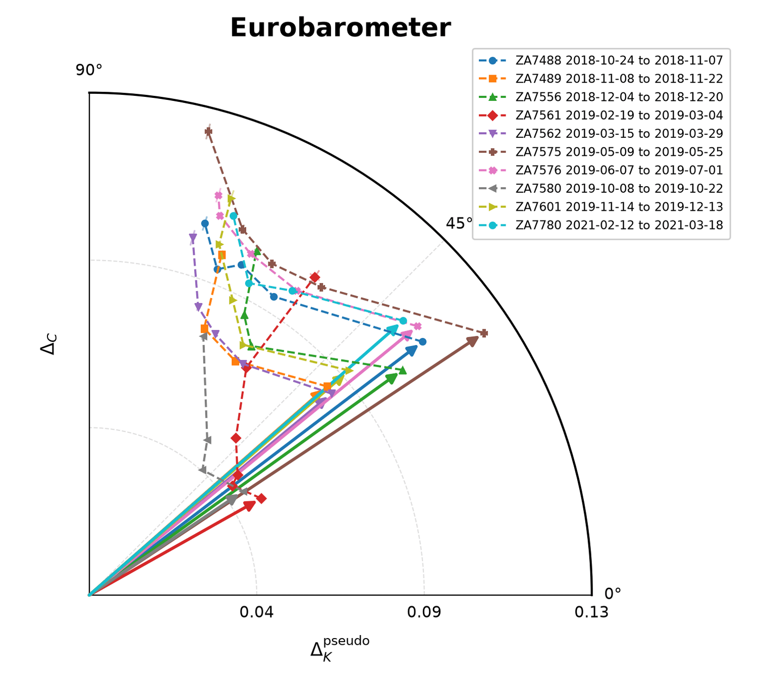
a
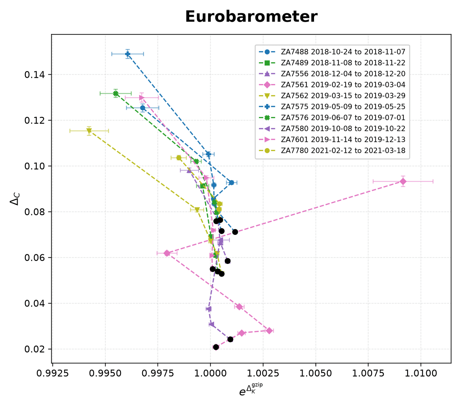
b
DIRECTION
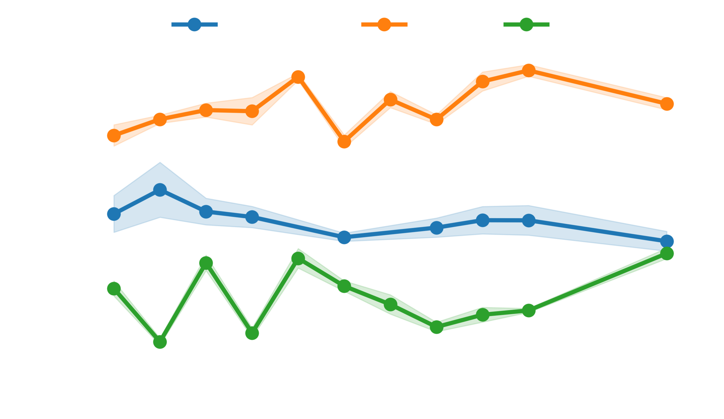
All ten arrows point within ≈30–43° in the (information drift, structural drift) plane.
MAGNITUDE
Arrow lengths range from ≈0.045 to ≈0.12; the 2021 wave, ZA7780, lies within the 2018–19 range.
KOLMOGOROV DRIFT
Within ≈ ±0.006 for every wave except one ZA7561 transition at ≈ +0.009.
RELATED FRAMEWORK
DTAG: digital twins of survey respondents
Characteristic Drift Spectra of Complex Systems
16 / 18
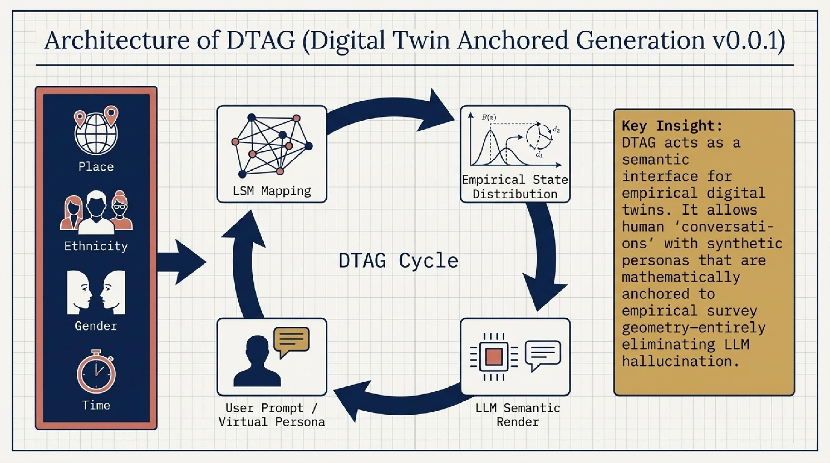
A survey-grounded synthetic respondent and synthetic survey simulator built on the same LSMs. Public research release v0.1.0-rc1 [12].
1
Persona → respondent state
An LLM maps persona text to survey-variable assignments that seed the state.
2
Question → survey variables
Embedding and LLM matching against a survey-specific variable map.
3
Answer from the LSM
Responses come from the LSM’s conditional distributions given the current state; the LLM phrases them. State persists across questions.
4
Ideology tracking (GSS)
Position between liberal and conservative pole vectors, via the LSM’s q-distance:
RC1 coverage
GSS 2022: sex-specific LSMs; ideology tracking
GSS 2024: pooled LSM, persona-conditioned
WVS7: pooled LSM; country and year conditioning
Afrobarometer R1–R5: country conditioning (Nigeria, Ghana tested)
Eurobarometer: planned for a later release
Experiment harness: matched personas, forward, reverse and shuffled question orders, replicates, bootstrap CIs.
Proposed link to drift. A DTAG synthetic survey should be a re-realization of the real survey, not a reorganization of it: its drift spectrum should match the real one within finite-sample variation. The spectrum gives a task-free fidelity test.
OUTLOOK
Interpretation and next steps
Characteristic Drift Spectra of Complex Systems
17 / 18
A system-level measurement object whose primary distinction is between re-realization and reorganization.
Its only learning requirement is a stable estimate of the target-wise conditionals. LSMs are one available realization; alternative learners can be substituted without changing the definition of the spectrum.
ROUTES FOR QUANTIFYING FINITE-SAMPLE VARIABILITY AND CALIBRATING EACH COORDINATE
Matched-size refit nulls
Separate finite-sample variability from real drift at matched sample sizes.
Independent peeling rules
Recover the hierarchy with alternative peeling rules to test robustness.
Planted-change simulations
Inject known changes to map the sensitivity of each coordinate.
Alternative conditional learners
Swap the conditional learner to test dependence on the algorithm.
Alternative compressors
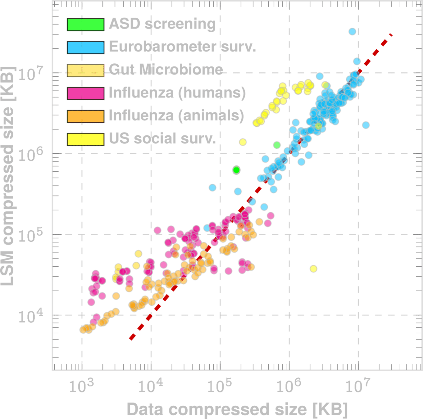
Test how Kolmogorov drift depends on the choice of gzip.
Observation-design controls
Separate changes in how data are collected from changes in the system.
ACKNOWLEDGMENT & REFERENCES
References
Characteristic Drift Spectra of Complex Systems
18 / 18
[1] J. G. Moreno-Torres et al., “A unifying view on dataset shift in classification,” Pattern Recognition 45(1):521–530, 2012.
[2] J. Gama et al., “A survey on concept drift adaptation,” ACM Computing Surveys 46(4), 2014.
[3] A. Gretton et al., “A kernel two-sample test,” JMLR 13:723–773, 2012.
[4] D. Lopez-Paz and M. Oquab, “Revisiting classifier two-sample tests,” ICLR, 2017.
[5] N. Sizemore et al., “A digital twin of the infant microbiome to predict neurodevelopmental deficits,” Science Advances 10(15):eadj0400, 2024.
[6] K. Wu, F. Li, and I. Chattopadhyay, “Emergenet: A digital twin of influenza A evolution for vaccine strain forecasting and emergence risk assessment,” Military Medicine, usag255, 2026.
[7] NORC at the University of Chicago, “General Social Survey 2021 codebook,” 2021.
[8] NORC, “General Social Survey 2022 codebook,” 2023.
[9] NORC, “General Social Survey 2024 codebook,” release 2, 2025.
[10] NORC, “Sequential data collection designs in the General Social Survey,” GSS Methodological Report 140, 2025.
[11] M. Li et al., “The similarity metric,” IEEE Trans. Information Theory 50(12):3250–3264, 2004.
[12] DTAG: Digital Twin Attitude Generator, v0.1.0-rc1, github.com/zeroknowledgediscovery/DTAG, 2026.
[13] Eurobarometer survey data, GESIS Data Archive, studies ZA7488–ZA7780.
Correspondence: ishanu_ch@uky.edu
Acknowledgment. This material is based upon work supported by the Defense Advanced Research Projects Agency (DARPA) under Agreement No. HR0011-26-3-E016. The views, opinions, and/or findings expressed are those of the authors and should not be interpreted as representing the official views or policies of the Department of Defense or the U.S. Government.
reliten |
gunlaw |
abany |
--- |
grass |
|
|---|---|---|---|---|---|
Person 1 |
|||||
Person 2 |
|||||
--- |
|||||
Person m |
observables
samples
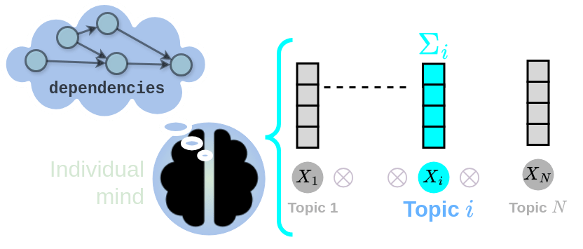
Distributions over alphabet \(\Sigma^i\)
Individual Predictor (CIT)
cross-talk
Tension between predicted and observed distribution drives change
Example
GSS topic: There should be more gun-control
\(\psi^i\)
strongly agree |
agree |
neutral |
disagree |
strongly disagree |
\(\phi\) estimates \(\psi\)
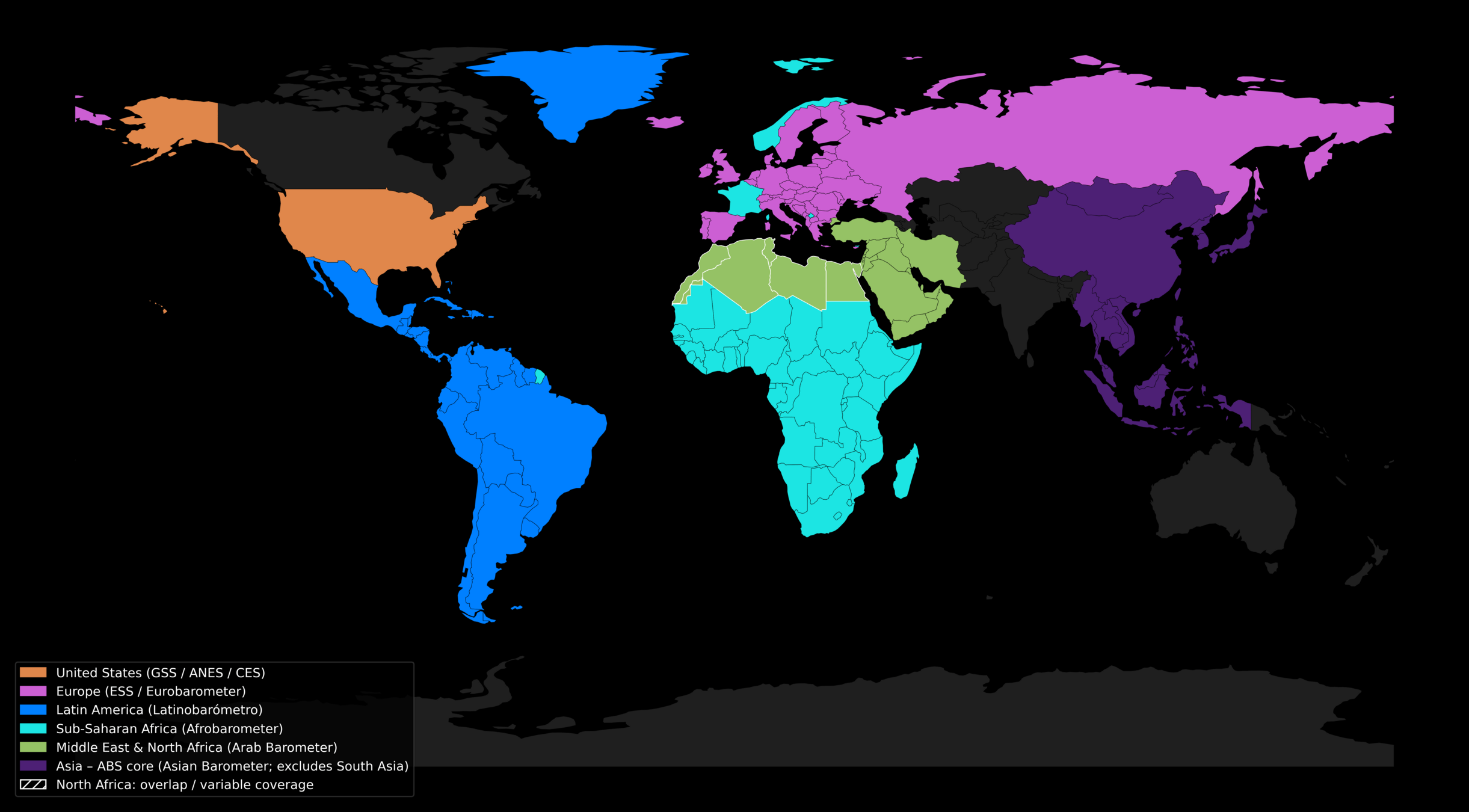
Examples: GSS, ANES, WVS, ESS, Eurobarometer, Afrobarometer, Asian Barometer etc
group
individual
estimate is always a non-empty non-degenerate distribution
missing observation
where \(D_{JS}(P\vert \vert Q)\) is the Jensen-Shannon divergence.
This bound connects ``closeness'' of samples to the odds of perturbing from one to the other, bridging geometry to dynamics
(Sanov's Theorem, Pinkser's Inequality)
\(\psi\)
\(\psi'\)
\(\theta\)
"spatial average": average of all plausible worldviews or states
* Sizemore, Nicholas, Kaitlyn Oliphant, Ruolin Zheng, Camilia R. Martin, Erika C. Claud, and Ishanu Chattopadhyay. "A digital twin of the infant microbiome to predict neurodevelopmental deficits." Science Advances 10, no. 15 (2024): eadj0400. https://www.science.org/doi/full/10.1126/sciadv.adj0400
persistence probability
Central to Model Drift Quantification
Start with opinion vector with all entries missing
This is a standard Physics construct, quantifying curvature of the underlying latent geometry
Easily computable in LSM framework!
Apply \(\phi^i\)
Random variable quantifying dispersion around the spatial average of worlviews
const. scaling as \(N^2\)
DatasetAccess modelLicense / use constraints (typical for research use)
General Social Survey (GSS) |
Open public download |
Free for research use; citation required; no redistribution of modified datasets |
American National Election Studies (ANES) |
Public-use + restricted-use tiers |
Public-use data freely available; restricted-use data requires application and secure handling |
Cooperative Election Study (CES) |
Public download (common content) |
Free for academic research; team modules may have additional citation or use constraints |
Eurobarometer |
Registration-based access (GESIS) |
Free for non-commercial research; user registration required; citation and compliance with GESIS terms |
World Values Survey (WVS) |
Registration-based download |
Free for non-commercial research; attribution required; redistribution restricted |
European Social Survey (ESS) |
Registration-based download |
Free for non-commercial research; strict citation and documentation compliance |
Latinobarómetro |
Controlled public access |
Use subject to project terms; citation required; redistribution limitations apply |
Afrobarometer |
Public download |
Free for research and policy use; attribution required; redistribution limited |
Arab Barometer |
Form-based access |
Free for non-commercial research; short request form; citation required |
Asian Barometer |
Application-based access |
Explicit permission required; usage and redistribution restrictions apply |
least easy
less easy
easy
World Value Survey (WVS) is global
\(\checkmark\) Overlapping survey datasets
Sample predicted distributions
perturbed state within \(\epsilon\) of \(\psi\)
Variable |
Masked |
Reconstructed |
|---|---|---|
spkcom |
allowed |
allowed |
colcom |
not fired |
not fired |
spkmil |
allowed |
allowed |
colmil |
allowed |
not allowed |
libmil |
not remove |
not remove |
libhomo |
not remove |
not remove |
reliten |
strong |
no religion |
pray |
once a day |
once a day |
bible |
inspired word |
word of god |
abhlth |
yes |
yes |
abpoor |
no |
no |
pillok |
agree |
agree |
intmil |
very interested |
very interested |
abpoorw |
always wrong |
not wrong at all |
godchnge |
believe now, always have |
believe now, always have |
prayfreq |
several times a week |
several times a week |
religcon |
strong disagree |
disagree |
religint |
disagree |
disagree |
Variable |
Masked |
Reconstructed |
|---|---|---|
spkcom |
allowed |
allowed |
colcom |
not fired |
not fired |
libmil |
not remove |
not remove |
libhomo |
not remove |
not remove |
gunlaw |
favor |
favor |
reliten |
no religion |
no religion |
prayer |
approve |
approve |
bible |
book of fables |
inspired word |
abnomore |
yes |
yes |
abhlth |
yes |
yes |
abpoor |
yes |
yes |
abany |
yes |
yes |
owngun |
no |
no |
intmil |
moderately interested |
moderately interested |
abpoorw |
not wrong at all |
not wrong at all |
godchnge |
believe now, didn't used to |
believe now, always have |
prayfreq |
several times a week |
several times a week |
2018 GSS individual samples
Definition
Sample neighborhood to impute missing data
}
2018 GSS out-of-sample reconstruction
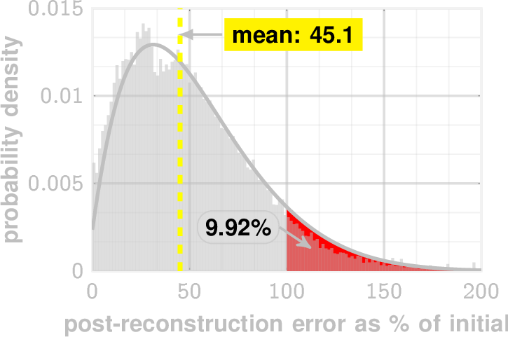
post-reconstruction error ratio (%)
LSM sampling: sampling the \(\epsilon\)-neighborhood of a state or worldview allows reconstruction of censored opinions
examples
Predictive ability of LSM quantified as ability to reconstruct censored out-of-sample opinions**
Null state (all missing observations)
Valid perturbations/ simulations
LSM sampling allows simulating opinion perturbations
Both Individuals and groups maybe modeled as digital twins\(\dag\)
The No-cheating Thorem: Generative models cannot cheat on complexity
Kolmogorov Complexity
Optimal Generative Model
compressed data representation
compressed model representation
Theorem
Conservation Law arising from the continuous symmetry of typicality*
Saturation relation:
Data Sufficiency Statistic \(\mu_0\)
We need LSM-sampling to calculate this
*Noether's Theorem
For every continuous symmetry of a physical system, there exists a corresponding conserved quantity
\(\checkmark\) 6. Explain how you will measure the accuracy of predicted structure emergence and data sufficiency.
How much more data do we need?
Data saturation
Data deficient
Needed
Current
Empirical Validation
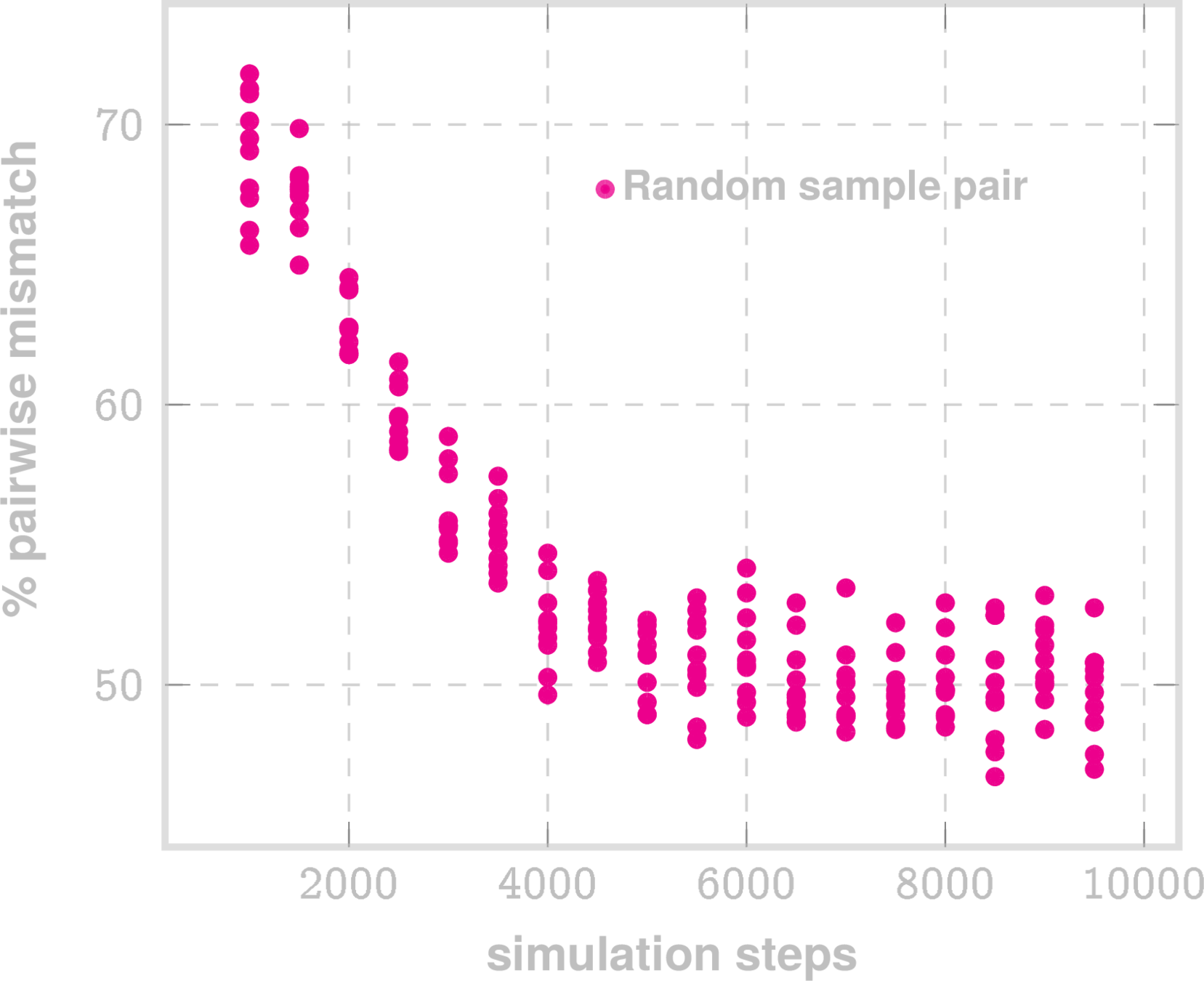
No Convergence
(~50% belief mismatch between pairs)
2018 GSS survey belief vectors simulated via LSM sampling
No ergodicity assumption: LSMs are built for non-ergodic systems
Sampling and simuation "remembers" the start point (No convergence), demonstrating non-ergodic learned structure
Local potential fields vary across the space
Potential wells may arise, driven by the dynamics at hand, not via assumptions
"change" is driven by non-equilibrium (dissonance)
Do new samples (survey respondents) still conform to the model?
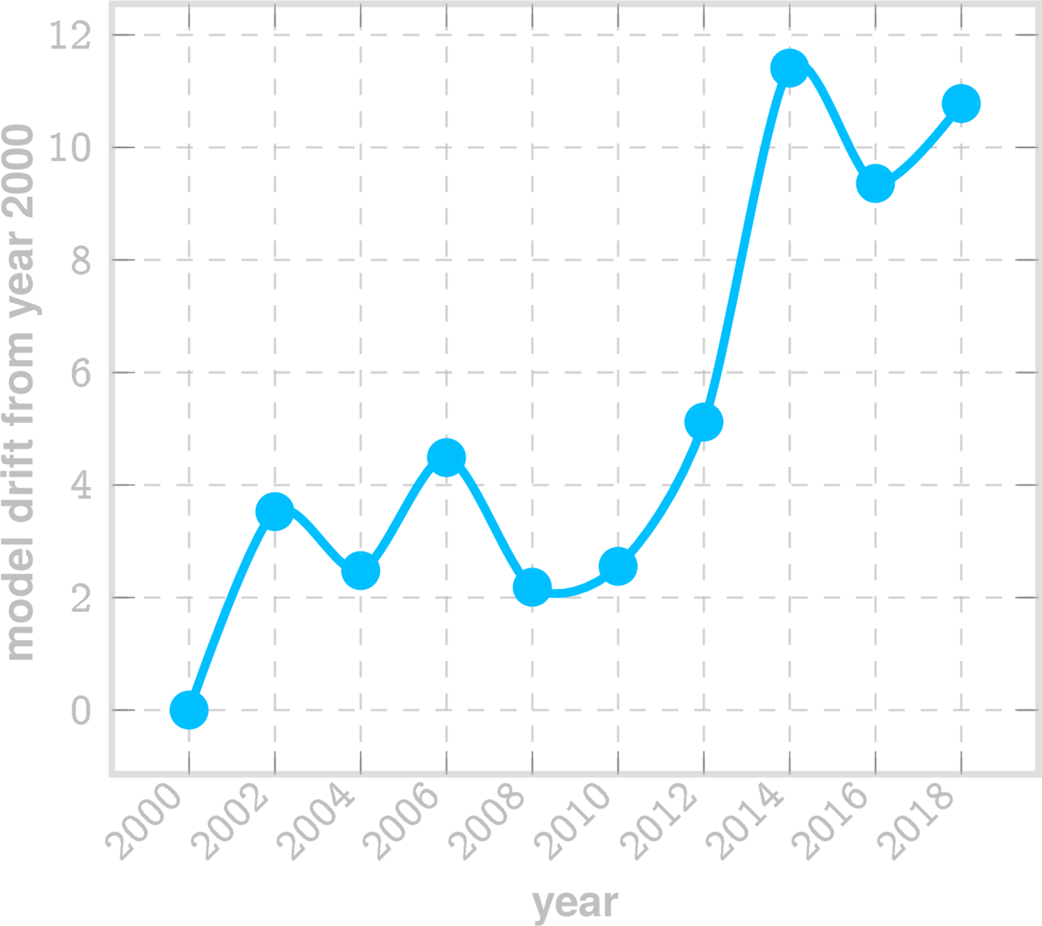
GSS Model drift
ergodic projection (all missing values)
A random belief state (with possibly missing entries)
random variable
normal variate
assess if \(\zeta\) is stationary: if not then new samples are not conforming to model
Example for GSS LSM inferred for year 2000
2018 GSS
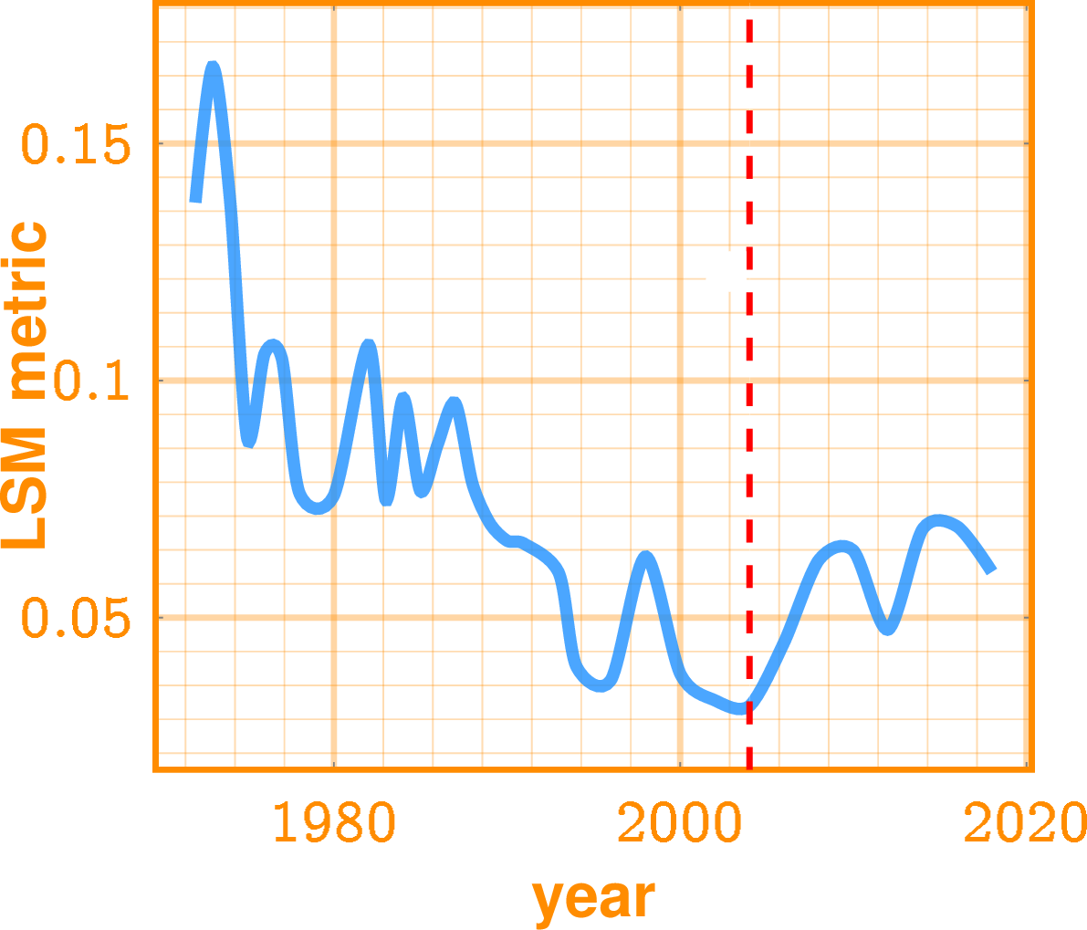
Polar separation over time
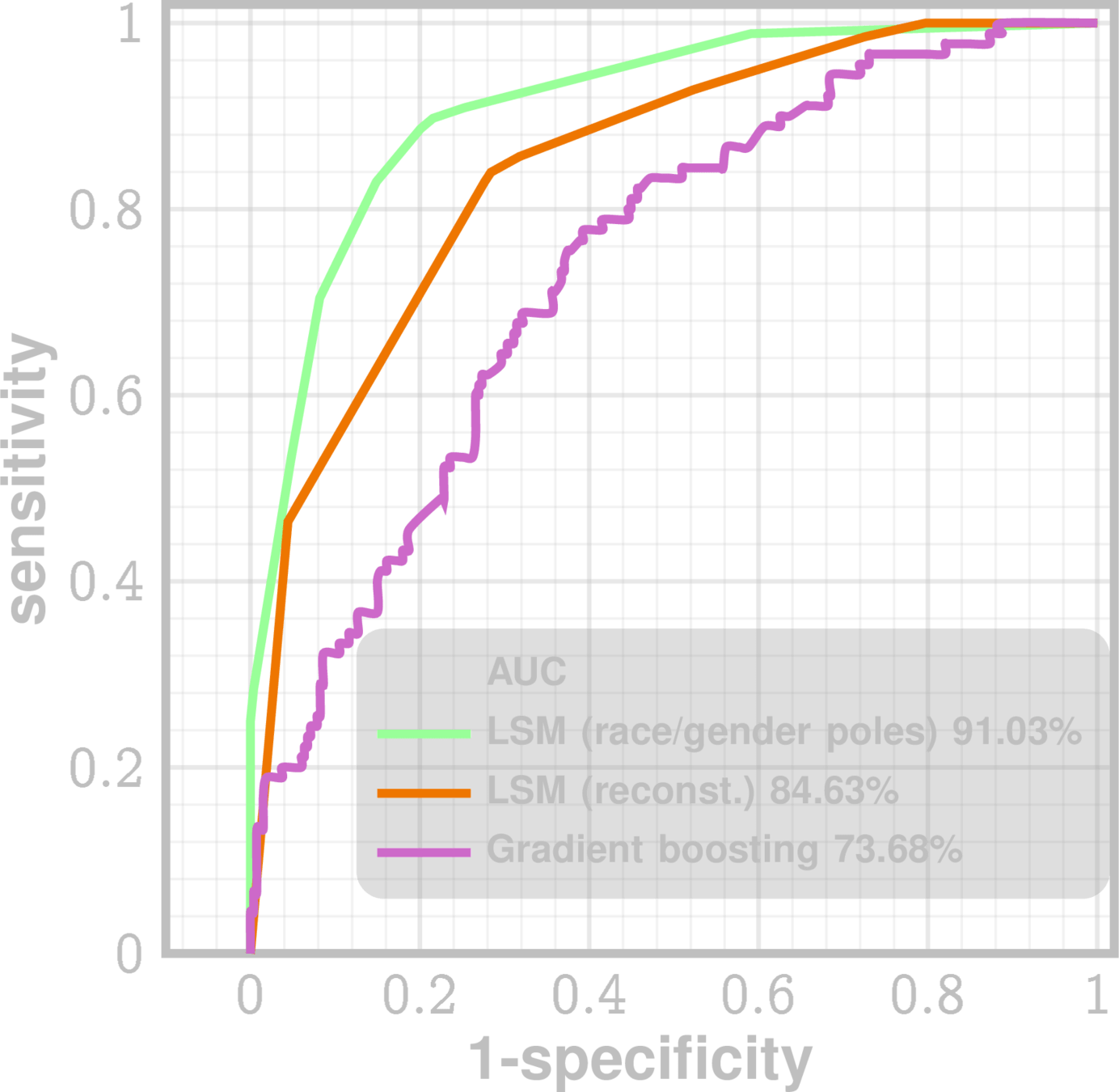
2016 Presidential Election Vote Prediction
2004
abany |
no |
yes |
abdefctw |
always wrong |
not wrong at all |
abdefect |
no |
yes |
abhlth |
no |
yes |
abnomore |
no |
yes |
abpoor |
no |
yes |
abpoorw |
always wrong |
not wrong at all |
abrape |
no |
yes |
absingle |
no |
yes |
bible |
inspired word |
book of fables |
colcom |
fired |
not fired |
colmil |
not fired |
not allowed |
comfort |
strongly agree |
strongly disagree |
conlabor |
hardly any |
a great deal |
godchnge |
believe now, always have |
don't believe now, never have |
grass |
not legal |
legal |
gunlaw |
oppose |
favor |
intmil |
very interested |
not at all interested |
libcom |
remove |
not remove |
libmil |
not remove |
remove |
maboygrl |
true |
false |
owngun |
yes |
no |
pillok |
agree |
strongly agree |
pilloky |
strongly disagree |
strongly agree |
polabuse |
no |
yes |
pray |
several times a day |
never |
prayer |
disapprove |
approve |
prayfreq |
several times a day |
never |
religcon |
strongly disagree |
strongly agree |
religint |
strongly disagree |
strongly agree |
reliten |
strong |
no religion |
rowngun |
yes |
no |
shotgun |
yes |
no |
spkcom |
not allowed |
allowed |
spkmil |
allowed |
not allowed |
taxrich |
about right |
much too low |
|
|
|
conservative pole
liberal pole
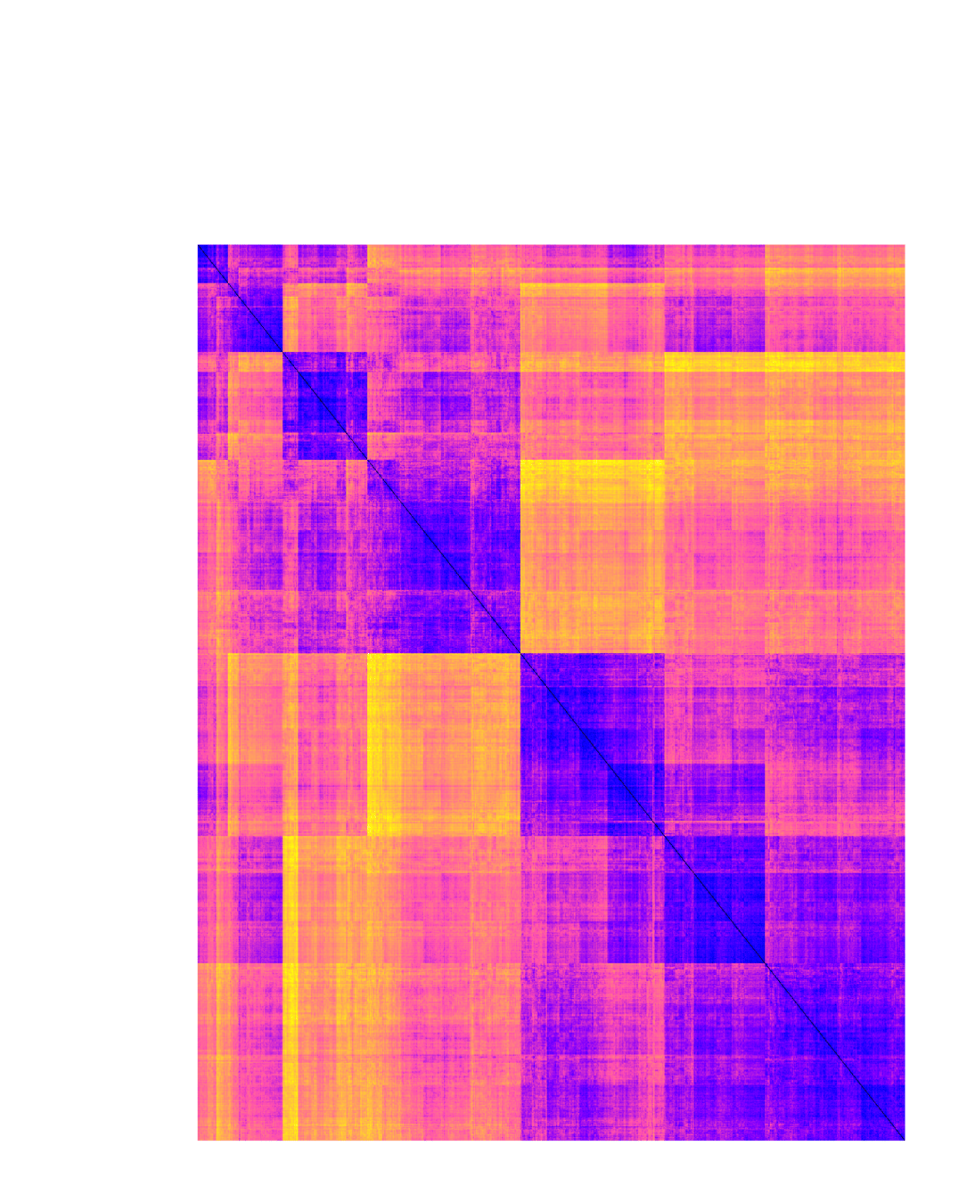
Clustering LSM distance \(\theta(x,y)\) between out-of-sample individuals
conservative
liberal
poles:
partial states aligning with extreme opposing worldviews
Compare across time and different GSS surveys
Derived features for individuals (ideology index)
Predict 2016 votes using ideology index
Emergent global structure
Define Lagrangian*
Via the Euler-Lagrange Equations\(^\dag\):
Over-damped Gradient flow Equation*
where \(-g^{km}\) is the inverse metric tensor
kinetic energy
state collapse
strongly agree
agree
neutral
disagree
strongly disagree
strongly agree
agree
neutral
disagree
strongly disagree
\(X_i\)
potential energy
* Einstein notation used
Goldstein, Herbert, et al. Classical Mechanics. 3rd ed., Pearson, 2002.
\(^\dag\)
Principle of stationary action
Local potential field eqn
How LSMs reflect and operationalize foundational social-scientific ideas
Belief about topic iii is expected to align with beliefs about other topics \(\displaystyle\psi^{-i}\).
Deviations are exponentially improbable \(\Rightarrow \) people/groups seek internal coherence.
Theory Link:
Cognitive consistency theory – Abelson et al. (1968)
Constraint satisfaction in beliefs – Read & Marcus-Newhall (1993)
Beliefs evolve to minimize tension between actual state and “expected” state.
Reflexive gradient flow — system reduces internal contradiction.
Theory Link:
Cognitive Dissonance Theory – Festinger (1957)
Homeostatic belief adjustment – Gawronski & Strack (2004)
Observing a belief changes it and affects all conditionals.
Direct encoding of feedback loops central to human systems.
Theory Link:
Reflexivity in social systems – Giddens (1984), Soros (1994)
Theory of mind / mutual modeling – Premack & Woodruff (1978)
Validation of Social Theory Questions:
Perception changes reality, which changes perception
The Constitution of Society
The Alchemy of Finance
Does a chimpanzee have a theory of mind?
Our system “wants” to reach a low-energy (low-dissonance) state — a direct computational analog of Festinger’s theory.
People strive to align beliefs and attitudes across related domains. Inconsistencies create cognitive discomfort, prompting adjustments across belief clusters to restore harmony.
|
Exploratory: Belief systems react measurably to exogenous events and shocks |
Exploratory: Cross-dependencies between beliefs have observable effects on societal resilience.
Is Polarization an Inevitable Attractor?
Social Identity Theory vs. Belief Proximity
A General Framework for modeling Complex Systems
Genomic database: Missing heritability problem
Personalized Clinical Digital Twin, Virtual Patients
Any structured interview, PTSD fabrication
Assess sysmptom data and co-pathologies
Predict future mutations; which animal strain is closest to jumping to humans
Mental health diagnosis
Microbiome Analysis**
Algorithmic lie detector
Viral emergence
Teomims
Opinion Dynamics
Darkome
Generative model of complex microbial ecosystems, and their impact on health and disease
Data requirements
Tabular data
Potentially large number of features/covariates (\(10^2 - 10^8 \))
Sufficient number of samples (\(10^3 - 10^6\))
Small number of longitudinal samples (currently, \( < 100\))
Limitation |
Mitigation / Response |
|---|---|
Conventional time series is currently out-of-scope |
Focus on cross-sectional interdependencies and belief geometry; time handled via drift |
LSMs model statistical interdependence, not causal mechanisms |
Use perturbation-based simulations to infer plausible influence pathways |
Limited by observed belief variables |
Integrate multiple surveys; use latent proxies and test sensitivity of digital twins |
Social theory connections and interpretability may be challenging |
Anchor dynamics with theory-driven constructs (e.g., ToM, cognitive dissonance) |
LSMs for complex systems
**preliminary study published (https://www.science.org/doi/10.1126/sciadv.adj0400)
By Ishanu Chattopadhyay
DARPA-EA-25-02-05-MAGICS-PA-025 University of Kentucky Kickoff