Networks and disease
Applications and inspiration from bighorn sheep
Pneumonia in bighorn sheep
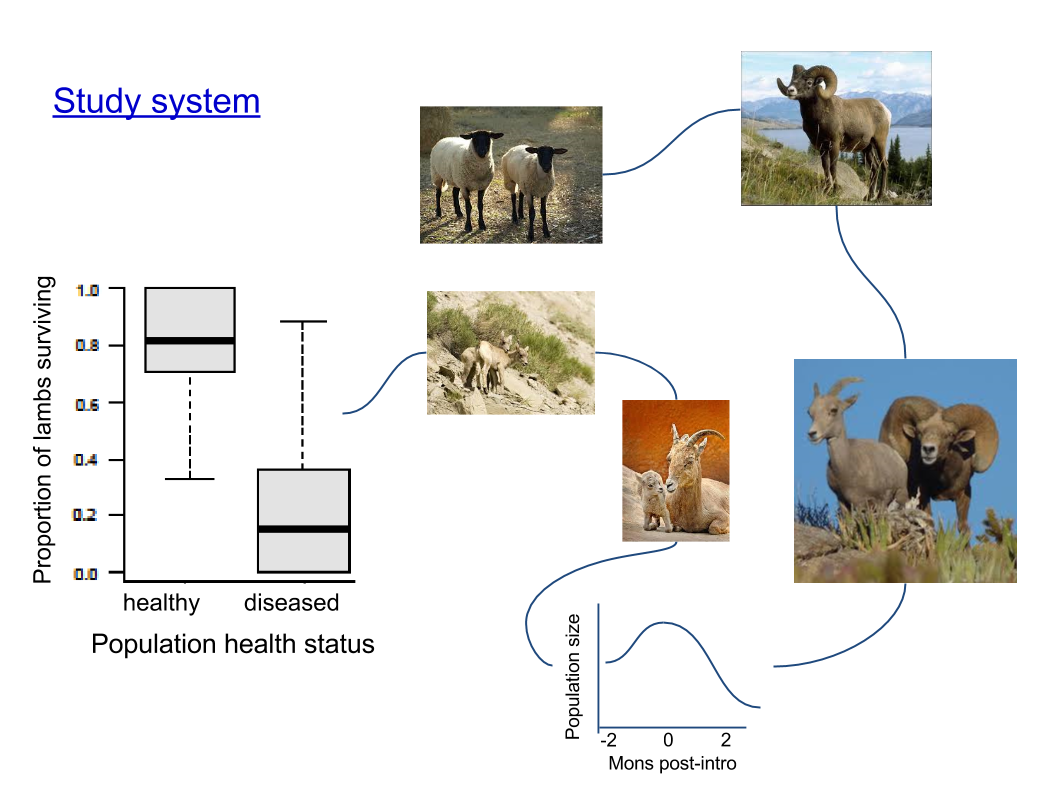
Cassirer et al. 2013, J Anim Ecol
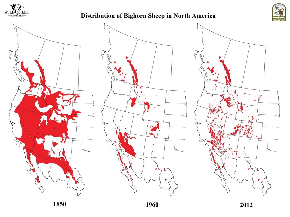
Source: Wild Sheep Foundation
Bighorn Health Consortium


Tom Besser,
Washington State
(vet microbiologist)
Frances Cassirer,
Idaho Dept Fish and Game
(wildlife biologist)
Raina Plowright
Montana State
Paul Cross, USGS
Pete Hudson,
Penn State
Conservation system
Challenges
- Leverage all available information
- Ask the right questions
Opportunities
- Long-term data
- Recently-established agent
Ph.D. program goals
1. Put forward the "most" urgent disease analyses based on existing data
2. Collect additional data on behavior and transmission (for states and funders)
3. Academic computing (for fellowship)
4. Basic science (for committee)
5. Technical support on collaborator projects
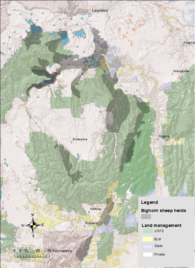
16 populations
Survey data since ~1970
Intensive study since 1996
500+ radiocollared animals
- mix VHF/GPS
- biweekly relocation interval (weekly in summer)
Lamb survival on ~700 lambs
Necropsies on
- >200 adults,
- >150 lambs
Longitudinal health sampling since 2011 in 3 populations

Pneumonia:
ephemeral or persistent?
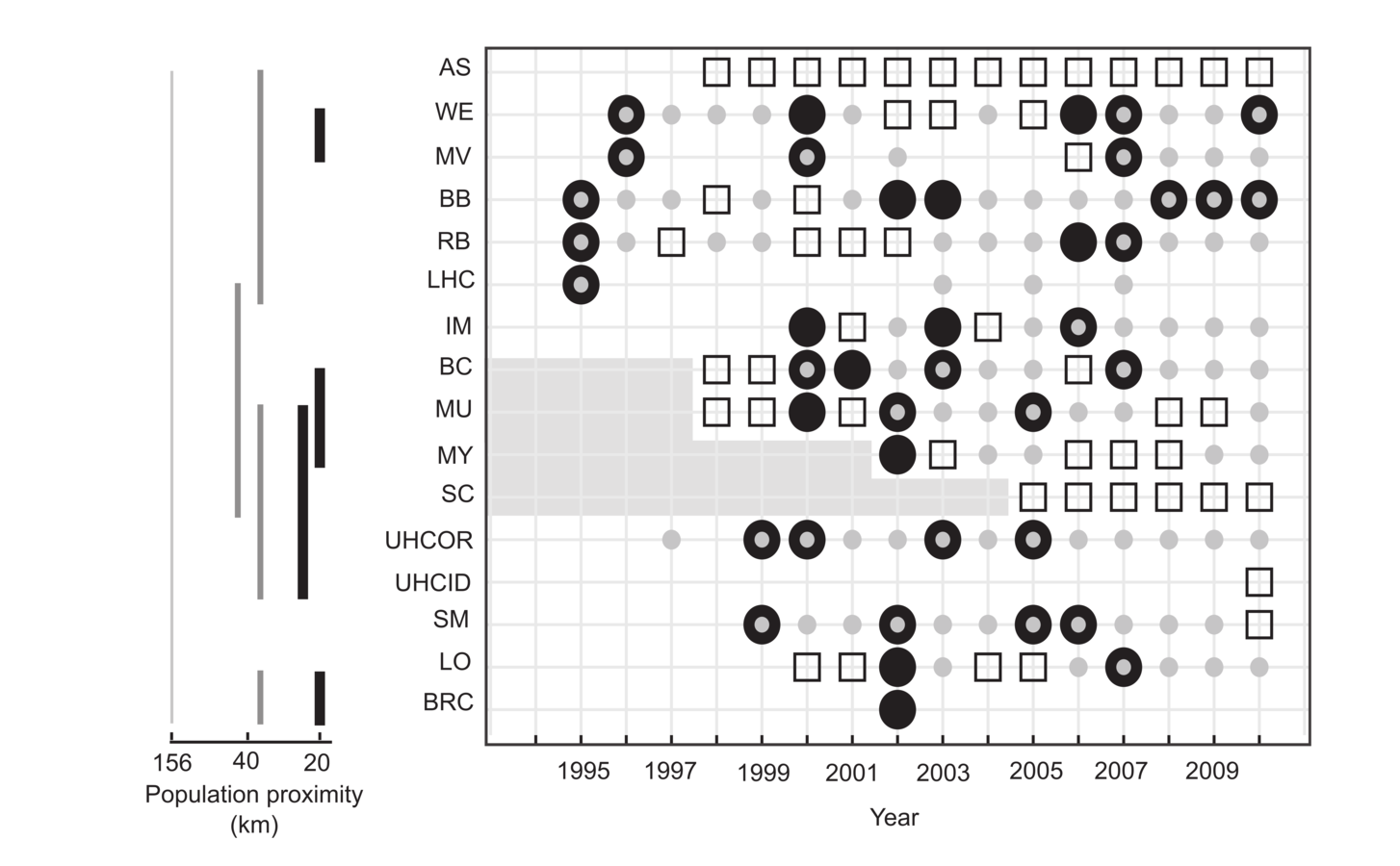
Healthy
Adult disease
Lamb disease
Populations
Cassirer et al. 2013, J Anim Ecol

Pathogen invasion stops population growth
Manlove et al. in review

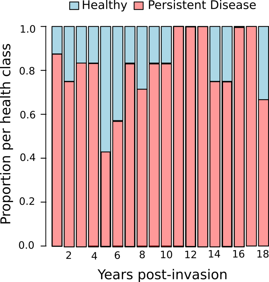
Manlove et al. in review
Years without documented pneumonia
Years with pneumonia
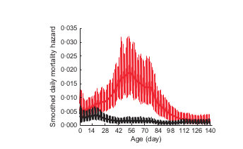
Age (days)
Smoothed daily mortality hazard
Cassirer et al. 2013, J Anim Ecol
Summer disease mortality asynchronous with typical ungulate juvenile mortality (over-winter)
Vital rates with and without disease
Objective:
combine multiple datastreams to draw inference to a single set of governing parameters
\mathbf{\sigma_{a}}, \mathbf{\phi_{a}}
\mathbf{Y_{1}} = f_{1}(\sigma_{a}, \phi_{a})
\mathbf{Y_{2}} = f_{2}(\sigma_{a}, \phi_{a})
(individual-level survival and reproduction)
(age-structured counts)
age-structured
survival
age-structured
P(wean a lamb)


Manlove et al. in review

Manlove et al. in review
What is the scale of transmission?
Are lamb mortalities well-mixed or localized to particular groups?


Well-mixed disease
Localized disease
=> low between-group variance
1) incomplete transmission, many sources
2) heterogeneous outcomes | infection
=> high between-group variance
1) localized infection
2) homogeneous outcomes | infection

Individuals
Sub-
populations
Years
Populations
Manlove et al. 2014 PRSB
Approach
1. Built networks using individual location data
2. ID'd groups (components)
3. Decomposed variance in lamb survival
log\left(\frac{p_{i}}{1 - p_{i}}\right) = subpop_{k[i]} + ewe_{j[i]}
subpop_{k} \sim N\left(year_{l[k]}, \tau_{subpop,PN} \times I(PN_{status})_{k} + \tau_{subpop,Healthy} \times (1 - I)PN_{Status})_{k}\right)
year_{l} \sim N\left(pop_{m[l]} + \delta I(PN_{Status})_{l}, \tau_{year,PN} \times I(PN_{status})_{l} + \tau_{year,Healthy} \times (1 - I)PN_{Status})_{l}\right)
pop_{m[l]} \sim N(0, \tau_{Pop})
ewe_{j} \sim N(0, \tau_{ewe})
i = individual lamb
j indexes ewes
k indexes groups in pops in years
l indexes pops in years
m indexes pops
year_{l} \sim N\left(pop_{m[l]} + \delta I(PN_{Status})_{l}, \tau_{year,PN} \times I(PN_{status})_{l} + \tau_{year,Healthy} \times (1 - I)PN_{Status})_{l}\right)
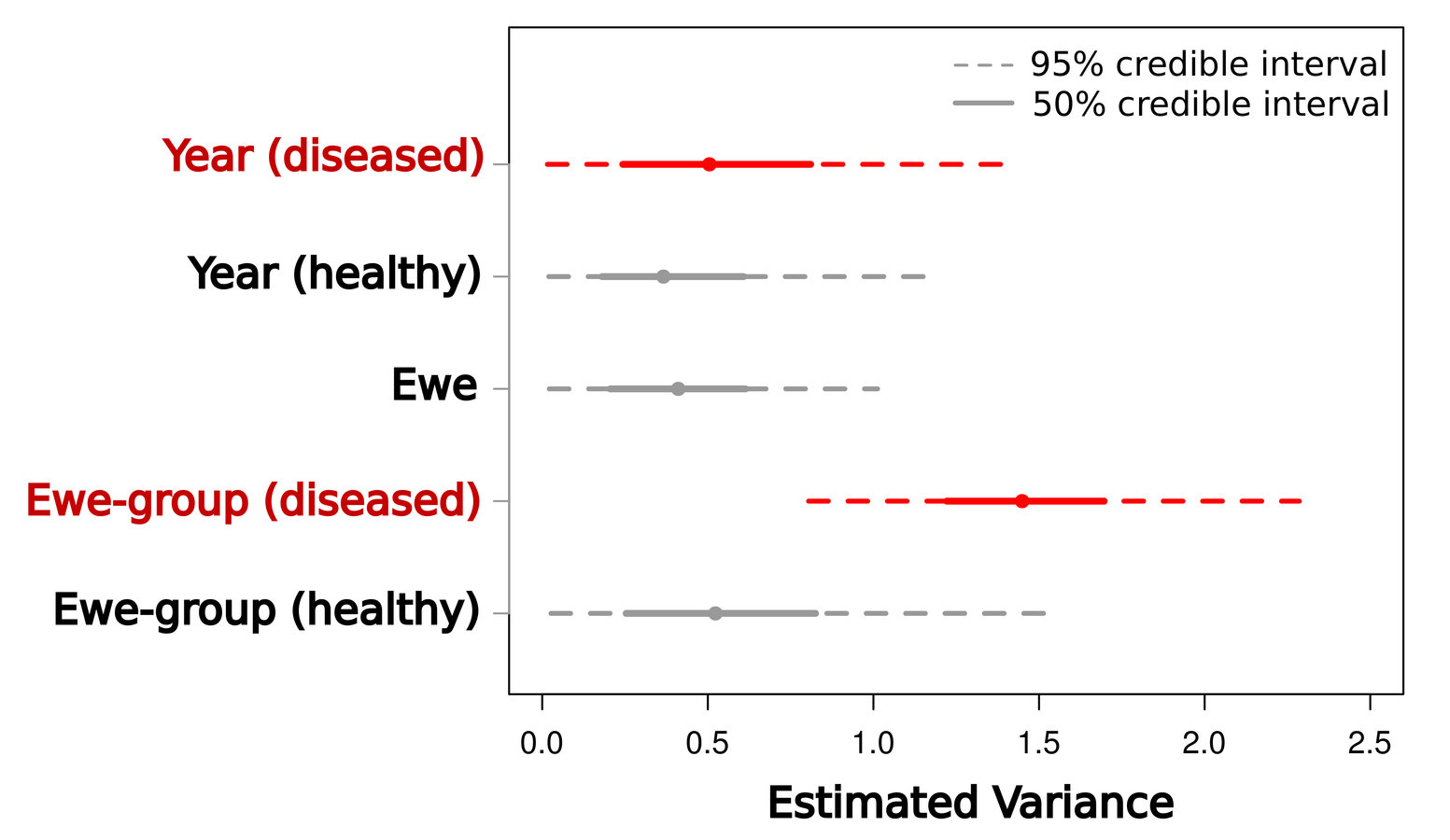
Manlove et al. 2014 PRSB
Evidence that transmission is localized within groups.
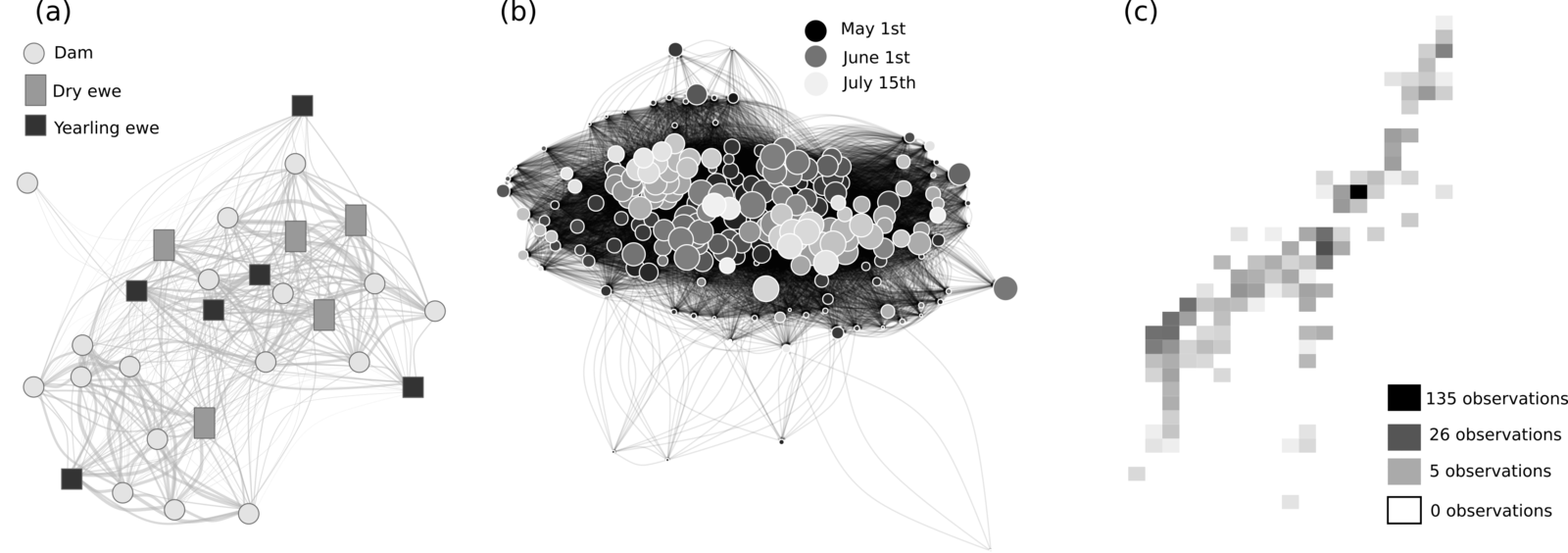
Follow-up question:
How does population size relate to group size?


Manlove et al. 2014 PRSB
(components = groups)
# groups increases with pop size...
... while group size remains stable
Disease may behave like it's FD
+
Relatively constant number of potentially infectious contacts
...no (or very low) CCS.
Localized, fairly complete transmission with consistent, severe effects
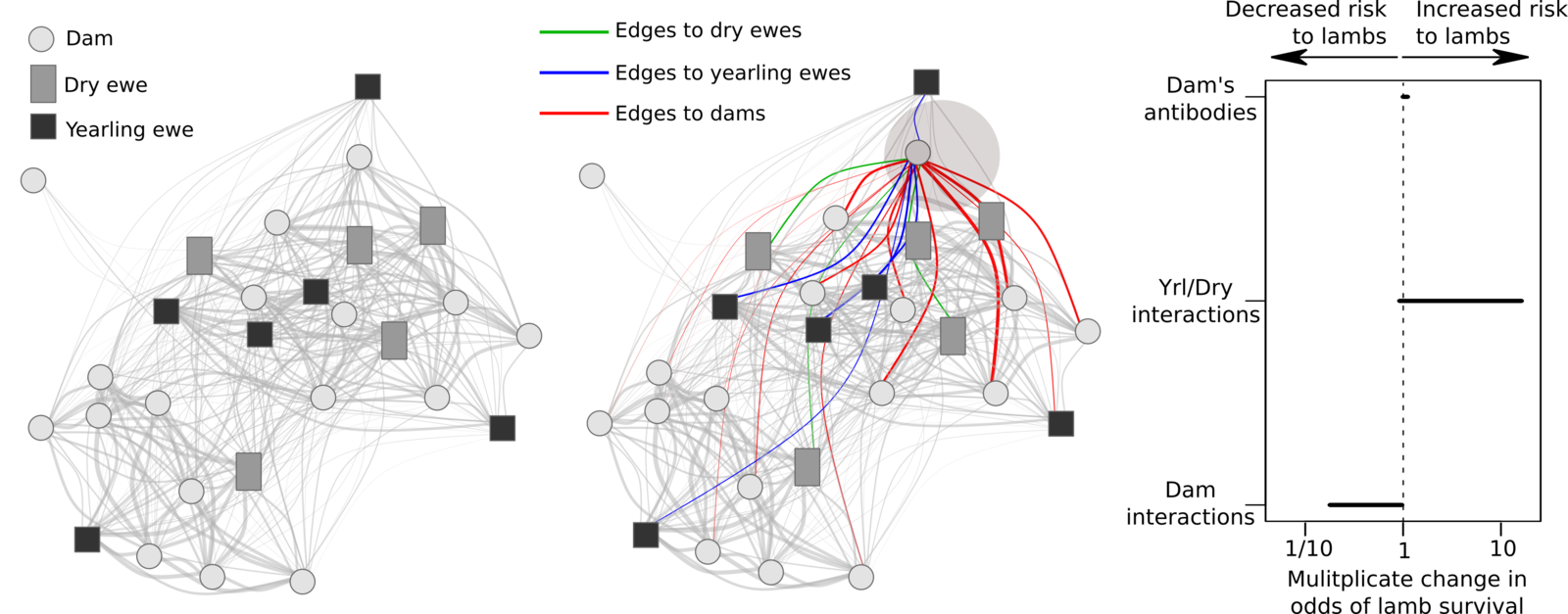
Behavior and transmission risk
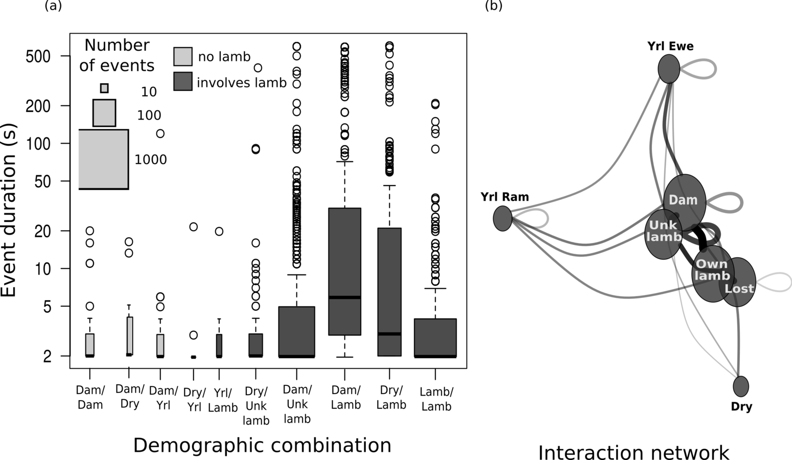

Association network
(Same place / same time)
(Direct touching)
Field data on bighorn behavior

Association centrality and interaction intensities
are not strongly correlated
Not all infecteds transmit.
Observation:
Can we use networks to infer something about P(transmission)?
Question:
Ideas from adaptive evolution
*Butler and King (2004) Am Nat


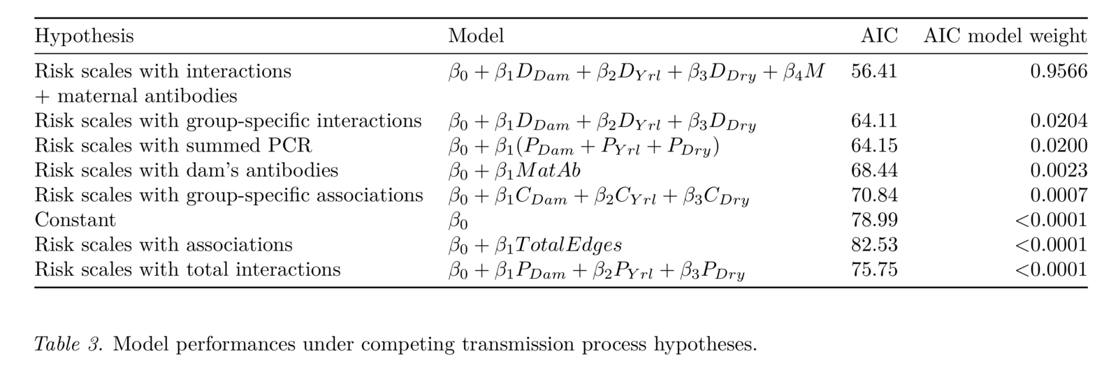
Manlove et al. in prep
Conceptualizing animal transmission networks
How do the constructions relate to one another?
How do we choose between them?
Different approaches produce different network topologies
Framework
Movement paths as triads in
(I, S, T)
Ecological analyses marginalize
(I, S, T)
Contacts occur at intersections in
(S, T)
Network construction methods use different projections of
(I, S, T)
Transmission occurs at intersections in some projection of
(I, S, T)
Movement paths as triads in
(I, S, T)
i \in (I^{*}: 1, ..., N)
D_{S^{*}} \subset \mathbb{R}^{d}
D_{T^{*}} \in \text{animal's lifetime}
(i, s, t) \sim f_{I^{*}, S^{*}, T^{*}}
Ecological analyses marginalize
(I, S, T)
| Analysis | Marginalized out | Density function |
|---|---|---|
| Home-range | ||
| Spatial spread | ||
| Individual survival | ||
| Occupancy |
T
f_{(I, S)} = \int_{t \in D_
T}f_{(I, S, T)}dt
f_{(S, T)} = \sum_{i \in I}f_{(I, S, T)}
I
f_{I, T} = \int_{s \in D_S} f_{(I, S, T)}ds
f_{S} = \sum_{i \in I}\int_{t \in D_T} f_{(I, S, T)}dt
S
I \text{ and } T
Contacts occur when
f_{(S, T)} \geq 2
f_{(S, T)} =
\begin{cases}
0 & \text{No animals present at this point in (S, T).}\\
1 & \text{One animal present.}\\
\geq 2 & \text{Two or more animals present: a contact.}
\end{cases}
Individual-specific contacts
I_1
with path
X_1 = \{I = I_1, S, T\}
I_2
with path
X_2 = \{I = I_2, S, T\}
Contacts between
occur at
I_1
I_2
and
X_1 \cap X_2 \in (D_S, D_T)
Network construction methods use different projections of
(I, S, T)
| Construction | Nodes | Edges | Density for intersections |
|---|---|---|---|
| Dynamic social networks | I | Together in S, T | |
| Static social network | I | Together in S, T |
|
| Home-range overlap networks | I | Overlapping home-ranges | |
| Circuit-like networks | S | Individual movements between sites | |
| Purely spatial networks | S | Spatial distance | ** |
(I, S, T)
(I, S)
(I)
** doesn't fit this framework very well....
(I, P)
where P = all occupied cells in (S, T)
Application to network choice
| Behavior pattern | Description | Examples | Dependence in (I, S, T) | Projection(s) |
|---|---|---|---|---|
| Territorial / spatially structured | Non-overlapping home ranges | wolves, prairie dogs, gerbils | ||
| Migratory | Time and space are correlated | Wildebeest, waterfowl, monarchs | ||
| Fission-fusion (strong bonds) | Groups are stable, but mix in space and time | Elephants, bison, giraffes | ||
| Fission-fusion (weak bonds) | Individuals mix in space and time | Elk, African buffalo | None |
(I, S)
(S, T) \text{ or } (I, T)
(S, T)
(I, S) \text{ or } (I, T)
(I, (S, T))
I \text{ or } (S, T)
(I, S, T)
In progress
Simulating animal movements and epidemics with varying
1. sociality
2. spatial preference
3. diffusion rate
across gradient of environmental : direct transmission
Building social, home-range, spatial networks
Simulating transmission on constructed networks
Measuring bias in predicted epidemic size and realized
under various network projections
R_{0}
deck
By Kezia Manlove


