Mathematical models of disease transmission
www.slides.com/keziamanlove/epimath
Who studies disease transmission, and how?
www.slides.com/keziamanlove/epimath
Olaf Hajek, nytimes
Contributing Disciplines
Within-host
Vet/Med
Micro/Immunol
"Omics"
Between- Host
Eco/Evo
Demography
Geographers
Prediction
Applied math
Statistics
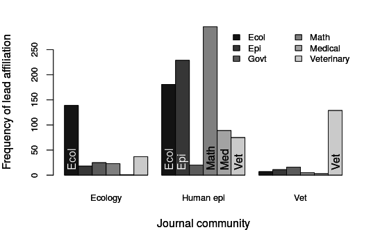
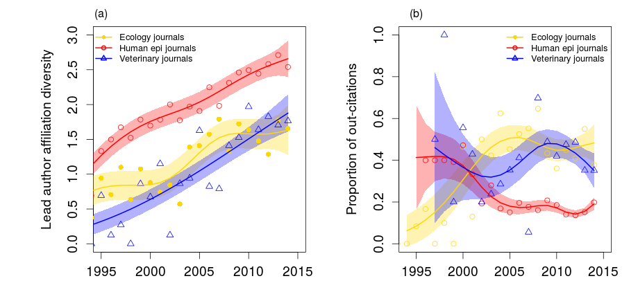
Where do papers on non-linear aspects of disease transmission get published?
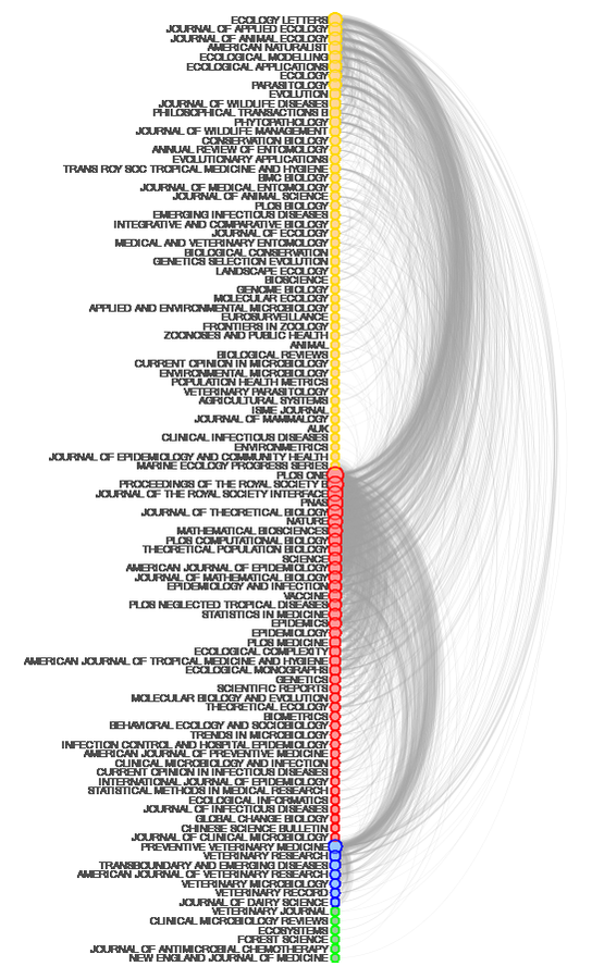
Where do papers on non-linear aspects of disease transmission get published?
K. Manlove et al., in prep
Ecology
Human Epi / Math
Vet
K. Manlove et al., in prep
Math. Biosci
PLoS Comp Biol
J Theor Biol
Theor Pop Biol
Where do papers on non-linear aspects of disease transmission get published?
K. Manlove et al., in prep
Math/Epi
Interface
History

Epi is not physics
Constraint # 1: Experimental ethics
Constraint # 2: Stochasticity is non-negligible
Consequences
1. Models remain very simple and general
2. Research emphasis on estimation/inference and "natural experiments"
Basic between-host model
Infected/
Infectious (I)
Susceptible (S)
Recovered (R)
States
I
S
R
\beta SI
\gamma
\mu
\mu
\mu
\mu = \text{Natural mortality}
\beta = \text{Transmission rate}
\gamma = \text{Recovery rate}
I
S
R
\beta SI
\gamma
\mu
\mu
\mu
\frac{dS}{dt} = -\beta SI - \mu S + \mu N
\frac{dI}{dt} = \beta SI - \left(\gamma + \mu\right) I
\frac{dR}{dt} = \gamma I - \mu R
\mu = \text{Natural mortality}
\beta = \text{Transmission rate}
\gamma = \text{Recovery rate}
Framework 1: Differential equations
Framework 2: Stochastic (Markov) process
| S | I | R | (D) | |
|---|---|---|---|---|
| S | ||||
| I | ||||
| R | ||||
| (D) |
1 - \beta SI - \mu
\beta SI
0
State at t + 1
State at t
0
1 - \gamma - \mu
\gamma
0
0
1 - \mu
\mu
\mu
\mu
0
0
0
1
I
S
R
\beta SI
\gamma
\mu
\mu
\mu
\mu = \text{Natural mortality}
\beta = \text{Transmission rate}
\gamma = \text{Recovery rate}
I
S
R
\beta SI
\gamma
\mu
\mu
\mu
\mu = \text{Natural mortality}
\beta = \text{Transmission rate}
\gamma = \text{Recovery rate}
\text{Transmission} = \text{(host contact rate)} \times \text{P(contact with infected)}
\times \text{P(Infection given contact with I)}
Transmission term,
\beta SI
\kappa
\propto \frac{I}{N} \text{ or } I
1 - c
\beta = -\kappa\log(1 - c)
I
S
R
\beta SI
\gamma
\mu
\mu
\mu
\mu = \text{Natural mortality}
\beta = \text{Transmission rate}
\gamma = \text{Recovery rate}
R_{0}
Basic reproductive ratio,
Expected number of additional "I"s created by a single "I" in an otherwise entirely "S" population
R_{0} = \frac{\beta}{\gamma + \mu}
\mu = \text{Natural mortality}
\beta = \text{Transmission rate}
\gamma = \text{Recovery rate}
R_{0}
Basic reproductive ratio,
| Disease | Mode of transmission | |
|---|---|---|
| Measles | airborne | 12-18 |
| Pertussis | airborne / droplet | 12-17 |
| Smallpox | Airborne droplet | 5-7 |
| HIV | Sexual contact | 2-5 |
| SARS | Airborne droplet | 2-5 |
| Influenza (1918) | Airborne droplet | 2-3 |
| Ebola (2014) | Bodily fluids | 1.5-2.5 |
R_{0}
R_{0} \leq 1 \Rightarrow \text{Limited transmission and eventual fade-out}
R_{0} > 1 \Rightarrow \text{Pathogen persistence}
Transmission and host density
Does transmission scale with population density?
...also depends on spatial scale
Sometimes no.
\beta \frac{SI}{N}
\beta SI
e.g., STDs
Sometimes yes.
"Density-dependent" transmission
"Frequency-dependent" transmission
aerosolized / fomite-driven transmission
Frequency- (FD) vs. Density- (DD) dependent Transmission
FD pathogens can drive the host extinct;
DD cannot.
(transmission eventually limited by too few S's)
I
S
R
Assumptions
1. Directly transmitted microparasites
2. Immunizing infections / life-long immunity
3. Well-mixed populations
4. Limited heterogeneity within compartments
Equilibrium Results
(Endemic disease)
Equilibria
\frac{dI}{dt} = \beta SI - \left(\gamma + \mu\right) I
\mu = \text{Natural mortality}
\beta = \text{Transmission rate}
\gamma = \text{Recovery rate}
\text{Equilibria at } I\left(\beta S - (\gamma + \mu)\right) = 0
I^{*} = 0
S^{*} = \frac{\gamma + \mu}{\beta} = \frac{1}{R_{0}}
Disease-Free
Endemic
I^{*} = \frac{\mu}{\gamma}\left(1 - \frac{1}{R_{0}}\right) = \frac{\mu}{\beta}\left(R_{0} - 1\right)
Herd immunity
System with vaccination rate and basic reproductive ratio
is dynamically identical to a system with
p
R_{0}
R_{0}^{'} = (1 - p)R_{0}
If high-enough proportion of pop is immune, pathogen will fade-out
Vaccination can manipulate downward
R_{0}
Age-Seroprevalence and
R_{0}
Seroprevalence: Proportion of population that has antibodies
to pathogen X (cumulative exposure; R + part of I)
For fully immunizing pathogens, Recovery is an absorbing state
A \approx \frac{1}{\mu(R_{0} - 1)}
Age at first infection (A) depends on infectiousness of pathogen ( ), and host life-span ( )
R_0
\mu
A \approx \frac{1}{\mu(R_{0} - 1)}
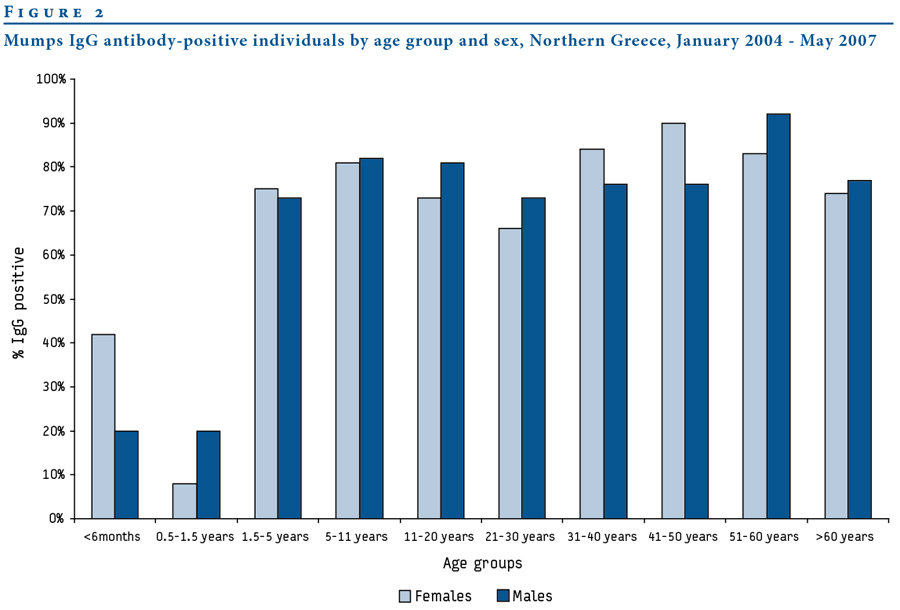
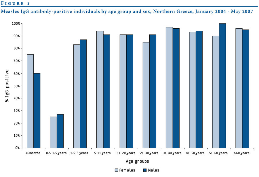
Fylaktou et al., Eurosurveillance, 2008
Measles
Mumps
R_{0}
R_{0}
12-18
4-7
Measles and Whooping cough
Assume constant pop size
Start with 3-D system
R(t) = N - S(t) - I(t)
So, system reduces to 2-D
\mu = \text{Natural mortality}
\lambda = \text{Force of infection}
\nu = \text{Recovery rate}
\frac{dS}{dt} = -\beta SI - \mu S + \mu N
\frac{dI}{dt} = \beta SI - \left(\gamma + \mu\right) I
\frac{dR}{dt} = \gamma I - \mu R
\frac{dS}{dt} = \mu - (\mu + \lambda(t))S(t)
\frac{d\lambda}{dt} = (\nu + \mu)\lambda(t)(R_{0}S(t) - 1)
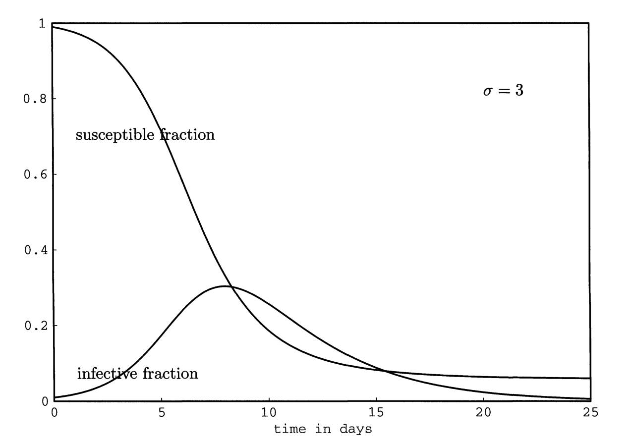
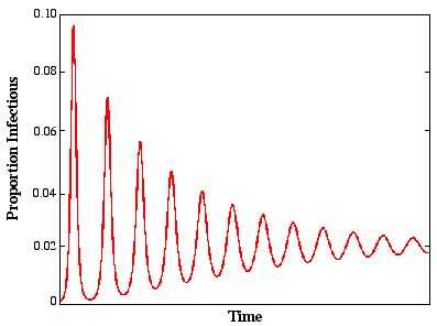
Damped Oscillator
\mu = \text{Natural mortality}
\lambda = \text{Force of infection}
\nu = \text{Recovery rate}
T \approx 2\pi\frac{L(\frac{1}{\nu} + \frac{1}{\sigma})}{R_{0} - 1}^{1/2}
L = \text{Host life expectancy}
\sigma = \text{Incubation rate}
Does this match reality?
Measles Fade-outs and Cycles
1. Critical community size:
Measles will "fade-out" in small pops, but not large ones
Continuous influx of susceptibles through births
2. Correlation between epidemic period and community size
Biennial periods in large communities; waiting time increases in smaller towns
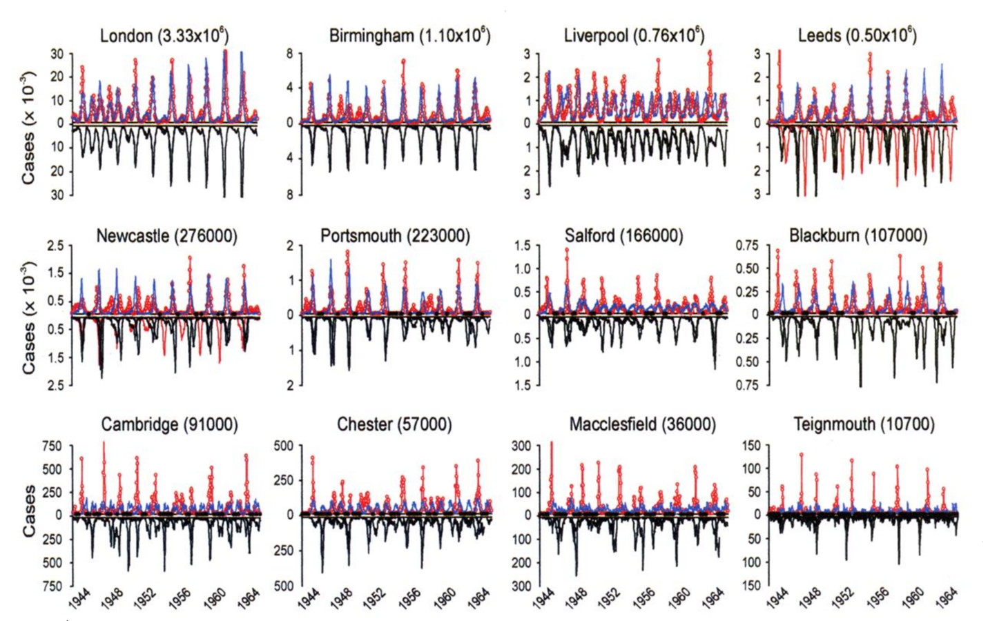
Pre-Vaccination Measles (UK)
Grenfell et al., 2001, Ecol Monogr
Don't look very damped....
How to explain "stable" oscillations?
1. Seasonal forcing from aggregation of school children
Pre-schoolers distinct from school-age peers
Problem: Too much fade-out
2. Realistic age structure
Pre-schoolers provide out-of-school contacts to get measles through trough
Added bonus: Sinusoidal forcing gets you chaos!
How transportable is that model?
1. Does model hold under varied birth pulse?
3. Does model hold for other childhood diseases?
2. Does model hold under vaccination?
Rohani et al., 2002, Am Nat
Measles in the UK
Post-WWII baby boom
Classic biennical cycles
Vaccination-era
Keeling, Rohani, Grenfell (2001) Physica D
Baby boom
Model re-creates observed change in measles period
over varied birth pulse and vaccination
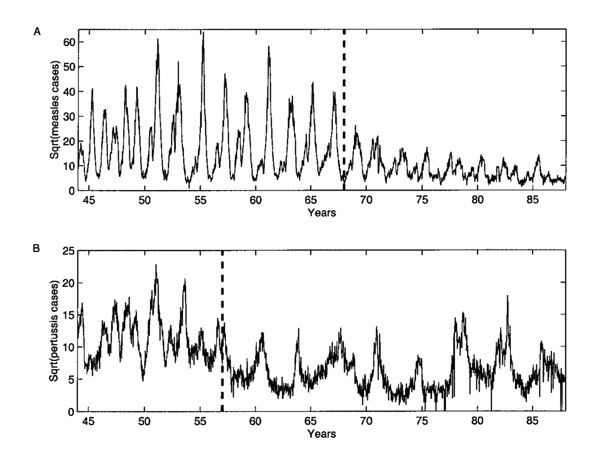
Rohani et al., 2002, Am Nat
Measles in the UK
Whooping cough
Annual outbreaks + 2-year epidemics
Post-vaccination 4-year cycles
Measles
Whooping Cough
In simulation, if you shift some S's and I's into R, system barely notices
System responds pretty dramatically if you move some S's and I's into R
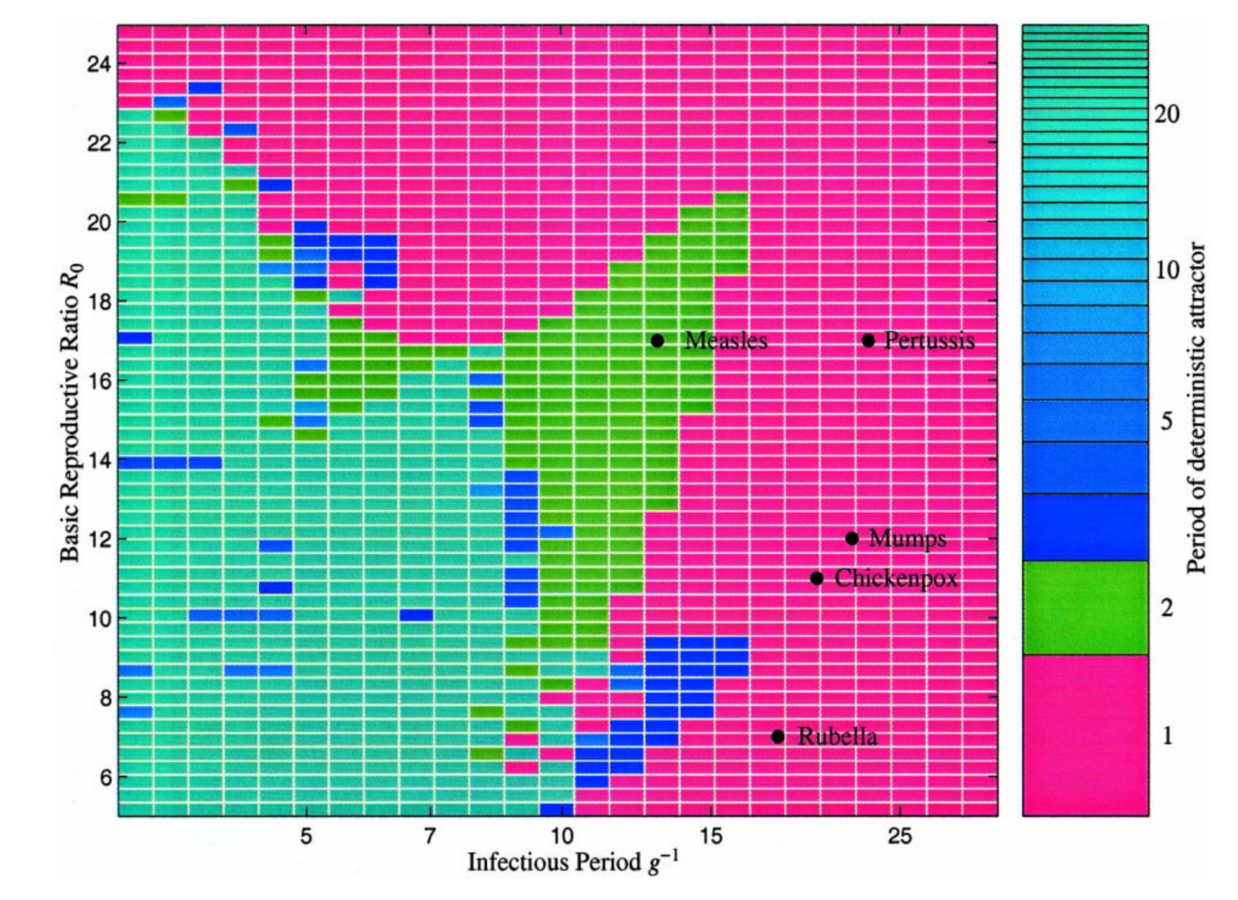
Do measles and whooping cough attractors differ in stability?
SIR models for measles and whooping cough
Do measles and whooping cough attractors differ in stability?
Compared dominant global Lyapunov exponents
Both systems have negative global Lyapunov exponents
=> stable, periodic attractor in both cases
(whooping cough slightly more negative than measles)
Both systems have similar local Lyapunov exponents
"Vaccination-like" perturbations (move some I's to R) have different impacts
Measles: transients return to the biennial attractor (so, robust)
Whooping cough: same magnitude of perturbation move trajectories off the attractor; you get multiyear periods of transient dynamics (so, sensitive)
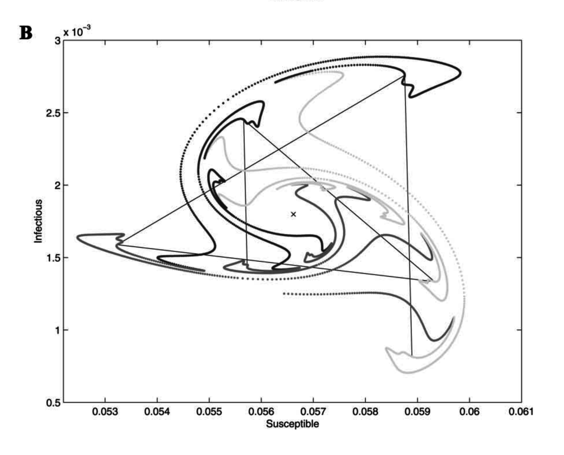
Measles
Whooping cough
Invasion orbits (very small I; almost all S)
Rohani et al., 2002, Am Nat
Whooping cough is really weird.
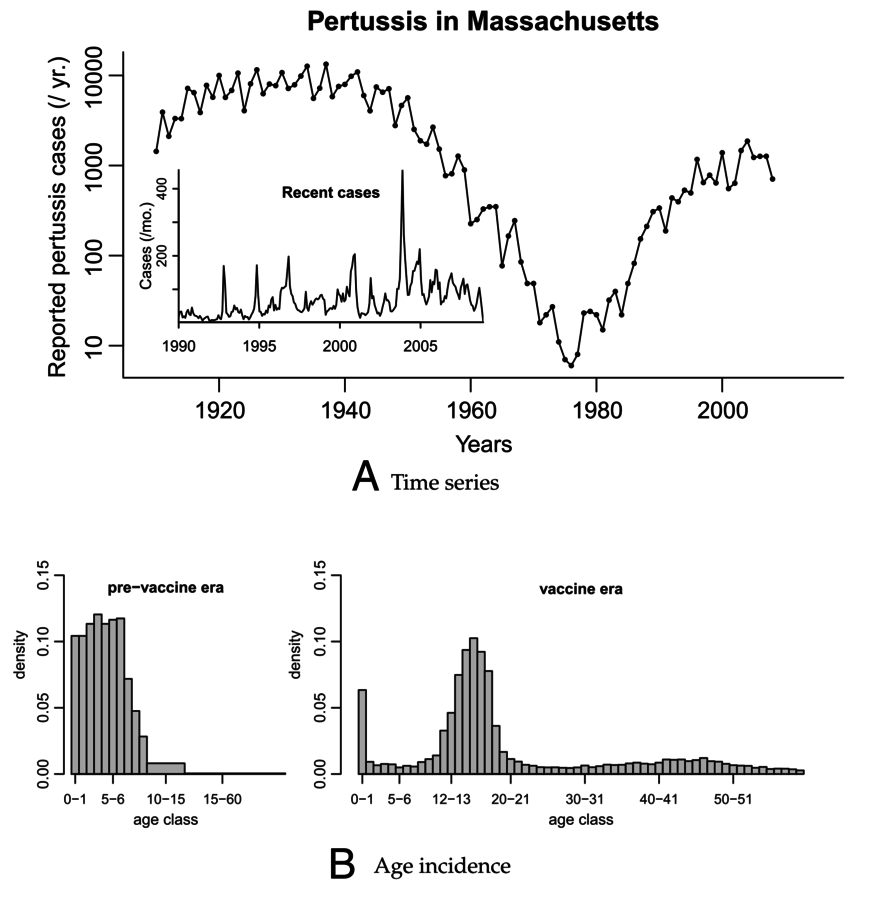
Lavine, King, Bjornstad (2011) PNAS
I
S
R
\beta SI
\gamma
\mu
\mu
\mu
\mu = \text{Natural mortality}
\beta = \text{Transmission rate}
\gamma = \text{Recovery rate}
W
(R is no longer an absorbing state)
\kappa \times \beta SI
\kappa = \text{Ease of boosting}
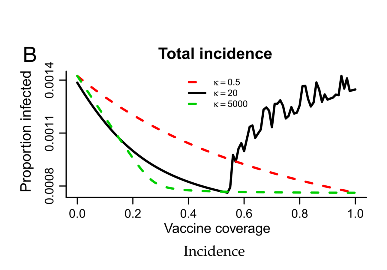
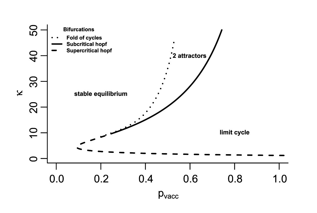
Why is whooping cough such a mess?
Hypothesis: Boosting through re-exposure
Lavine, King, Bjornstad (2011) PNAS
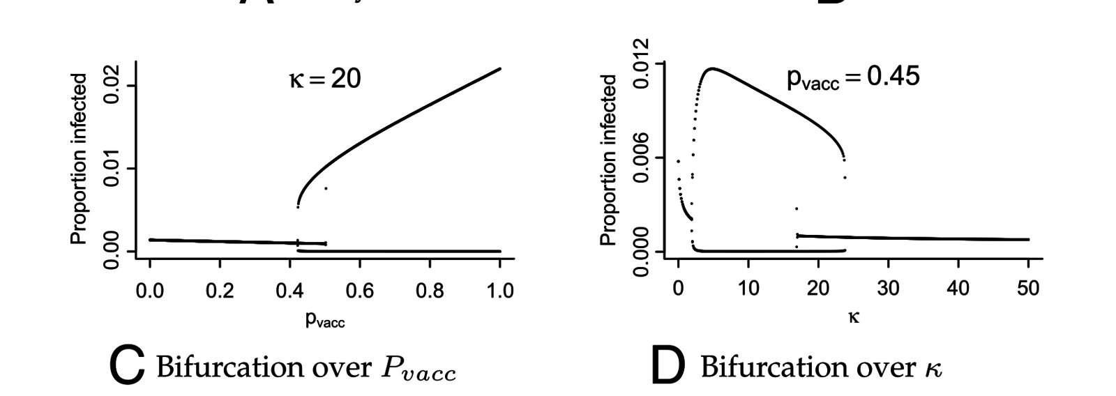
Lavine, King, Bjornstad (2011) PNAS
So, whooping cough boosting vaccinations for teenagers
Inference
State-space models
Approximate Bayesian Computation ("ABC")
Partially observed Markov Process Models
Current research foci
Super-spreaders
Basic tenet:
I is not homogeneous
SARS motivated
A few individuals apparently accounted for almost all of the transmission
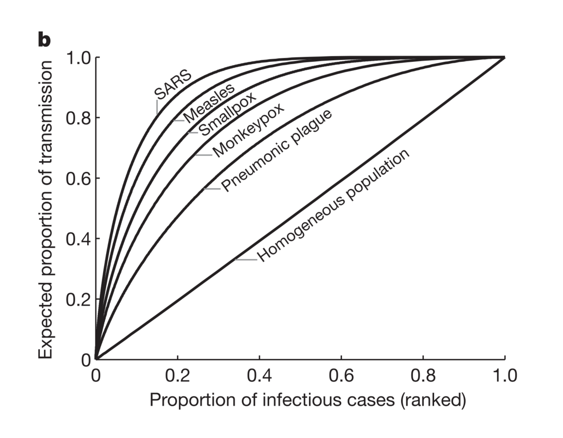
Lloyd-Smith et al., Nature, 2005
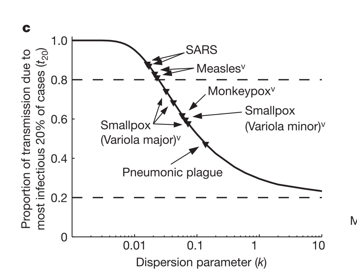
Focus: dispersion in # cases generated
Z = \text{RV representing number of } 2^{0} \text{ cases produced by a particular I}
\nu = R_{0} \Rightarrow Z \sim Pois(R_{0})
\nu \sim Exp() \Rightarrow Z \sim Geometric(R_{0})
\nu \sim Gamma\left(R_{0}, \kappa
\right) \Rightarrow Z \sim \text{Neg Bin}(R_{0}, \kappa)
\nu = \text{"individual reproductive number"} \sim \left(\mu = R_{0}\right)
\text{Var(Z)} = \frac{R_{0}}{1 + \frac{R_{0}}{\kappa}}
Increased dispersion in I led to more explosive, and rarer, epidemics
Cross-scale models
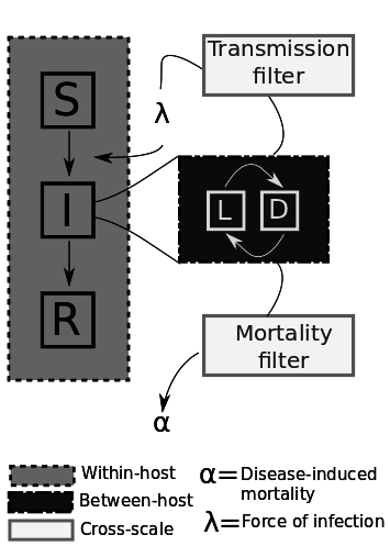
Two Questions
1. What happens in the host?
2. How do we map?
Two (non-mutually-exclusive) within-host models
Antigen-driven dynamics
- Predator-prey between immune system (D) and pathogen(L)
Network regulation model
- Internal feedbacks control host's immune response
\frac{dL(\tau)}{d\tau} = \rho L(\tau) - \frac{\nu L(\tau)^{2}D(\tau)}{\psi^{2} + L(\tau)^{2}}
\frac{dD(\tau)}{d\tau} = D(\tau)\frac{\phi\nu L(\tau)^{2}}{\psi^{2} + L(\tau)^{2}} - \epsilon D(\tau)
Holling Type III Functional response
Cross-Scale Considerations
Have to model age-of-infection for all I's
\Rightarrow{PDEs}
\frac{dS(t)}{dt} = \theta - \mu S(t) \int_{0}^{\infty}\beta(a)I(a, t)da
\frac{\partial I(a, t)}{\partial t} = -\frac{\partial I(a, t)}{\partial t} - \alpha(a)I(a, t)
I(0, t) = S(t) \int_{0}^{\infty}\beta(a)I(a, t)da
\theta = \text{birth rate}
\mu = \text{host mortality rate}
\alpha = \text{loss rate of individuals from I}
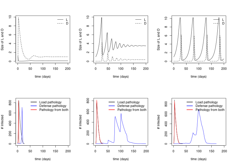
Within-host outcomes of pathogen invasion
1. Acute infection, followed by clearance
- Measles, Mumps, Rubella, Variola (Pox), Influenza
2. Recurrent disease (e.g., repeated growth and decay of pathogen population within the host)
- Herpes symplex virus, HPV, HIV, Tuberculosis
3. Inapparent / dormant infections (no symptoms; pathogen isn't detectable)
- Whooping cough (??)
4. Subclinical infections (no symptoms; pathogen is detectable)
Manlove, Cross, Plowright in prep.
Pathogen clearance
Pathogen persistence
Pathogen cycling
Consider 3 maps from within- to between
1. Transmission / mortality depend only on Load (L)
2. Transmission / mortality depend only on Defense (D)
3. Trans / mort depend on some combination of L and D
Manlove, Cross, Plowright in prep.
Pathogen clearance
Pathogen persistence
Pathogen cycling
Social network theory and contacts
Wrap-up
1. Epidemiological modeling is fundamentally x-disciplinary
2. Historic challenge: identifying deterministic vs. stochastic aspects of system
3. Current mathematical foci:
- x-scale modeling
- spatial spread
4. Current statistical foci:
- Non-linear series data (esp. hierarchical modeling structures)
- Spatiotemporal data analysis
- Hierarchical inferential schemes
Questions?
www.slides.com/keziamanlove/epimath
Math models for epi
By Kezia Manlove
Math models for epi
Applied math seminar talk


