






What is Matrix Hydrodynamics?

Klas Modin

FoCM, Vienna, 2026

Starting January 1st, 2027, the

Journal of FoCM is published

by EMS Press under a

Subscribe-to-Open (S2O) model

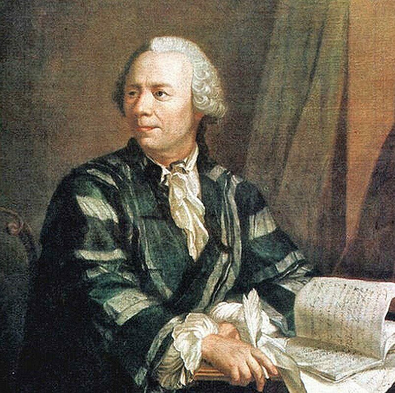
270 Years Towards a More Perfect

Theory of Fluid Motion

...

it is not the principles of mechanics we lack, but only analysis, which is not yet sufficiently developed. Thus, we clearly see what discoveries we need to make before we can arrive at a more perfect theory of fluid motion.

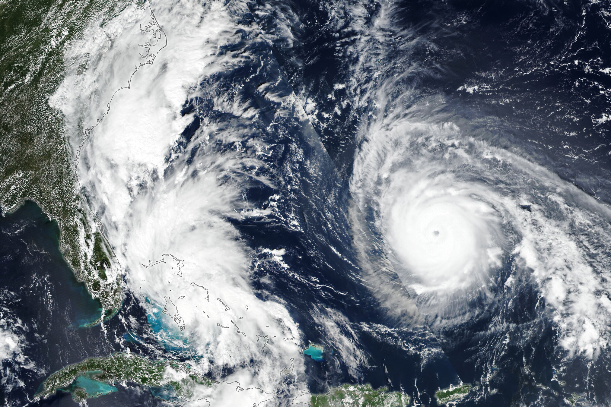
Why Study 2d Euler?

(c) NASA, 2025

Imelda

Humberto

(c) ECMWF, 2025

Why Study 2d Euler?

[H. Kelley, Phys. Fluids, 2017]

Why Study 2d Euler?

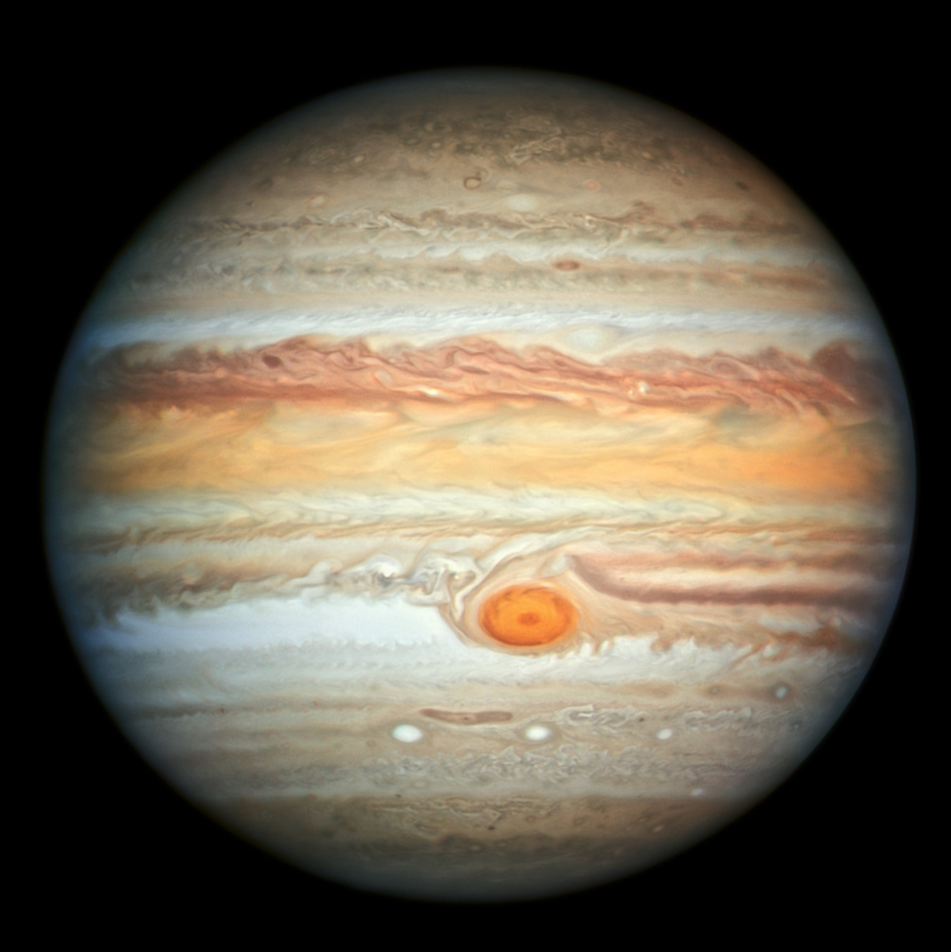
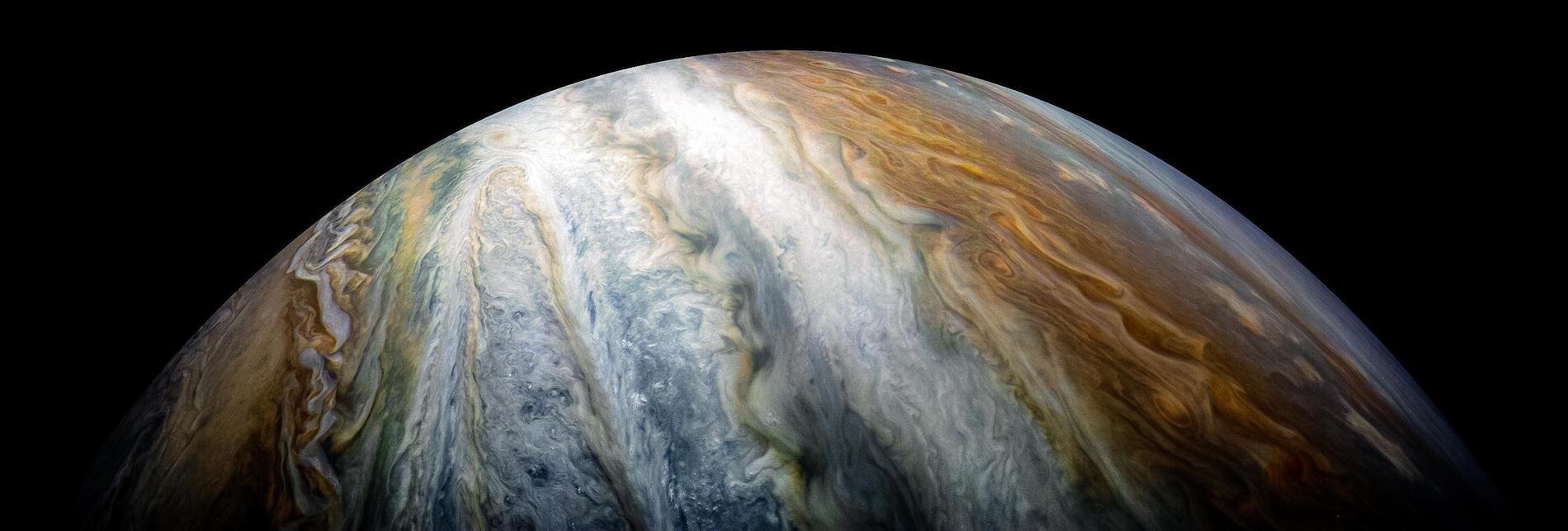
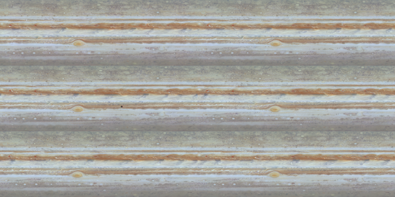
(c) NASA (Hubble + Juno mission) 

Why Study 2d Euler?

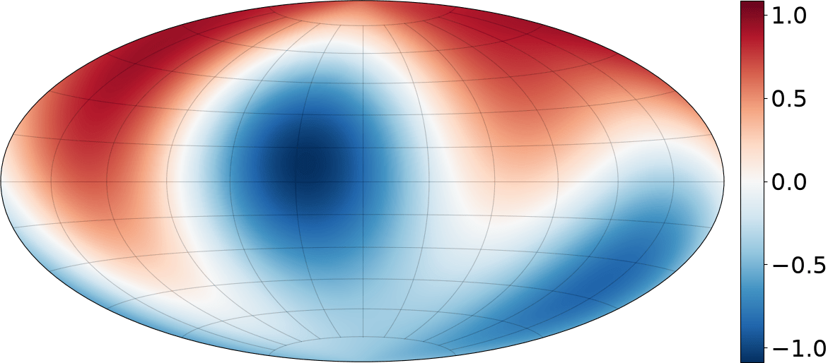
A continuous medium deprived of its physical properties (elasticity, thermal and electrical conductivity, and so on) still retains a definite position in space and still interacts through the mutual pressure of its parts due to Aristotle’s principle that two bodies cannot occupy the same space. Amazingly, it is these elementary interactions that cause the most intricate behavior, including turbulence.

Victor Yudovich

\dot v +\nabla_v v = -\nabla p
\operatorname{div}v = 0

The Jewel of 2d Hydrodynamics

\dot v +\nabla_v v = -\nabla p
\operatorname{div}v = 0
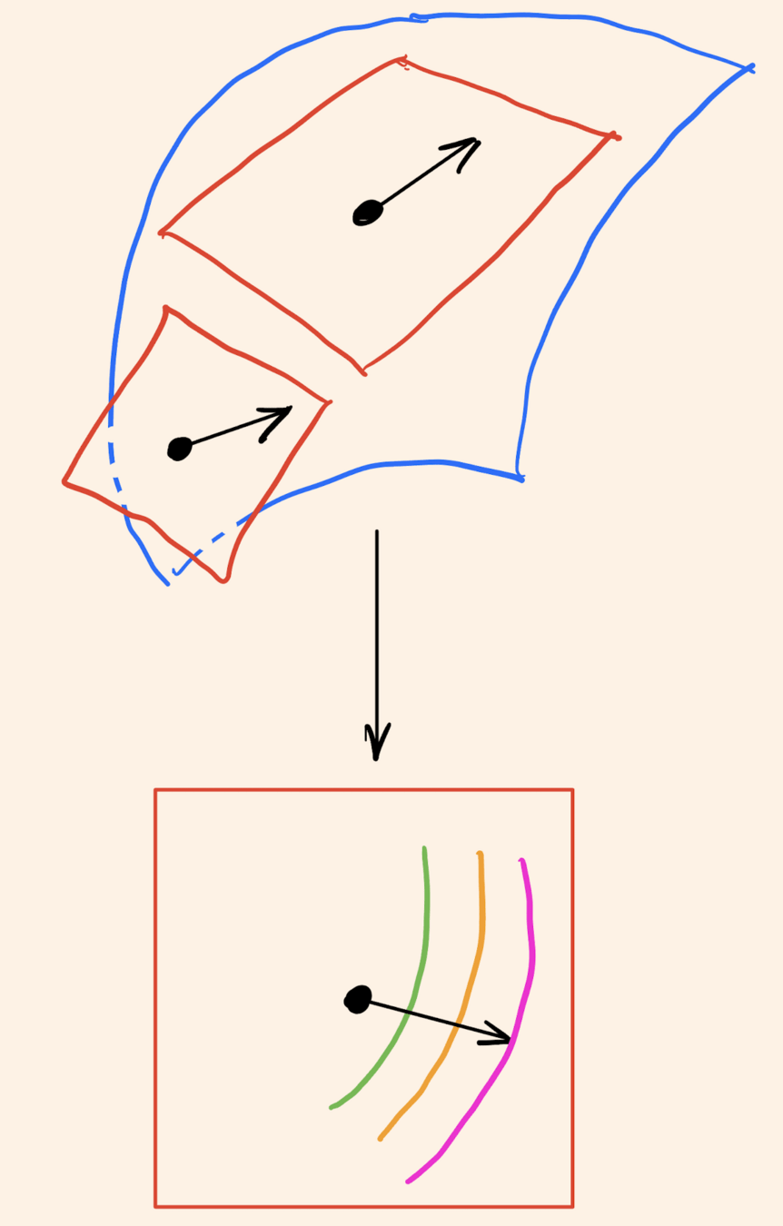
\displaystyle \dot \omega + \operatorname{div}(\omega v) = 0
\quad \omega + \Delta\psi = 0
\quad v = \nabla^\bot\psi
\frac{\partial}{\partial t}\underbrace{\operatorname{curl}v}_\omega +\operatorname{curl}\nabla_v v = -\underbrace{\operatorname{curl}\nabla p}_0

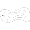
level-sets of \(\omega\)

\(v\)

Matrix Approach

by Zeitlin

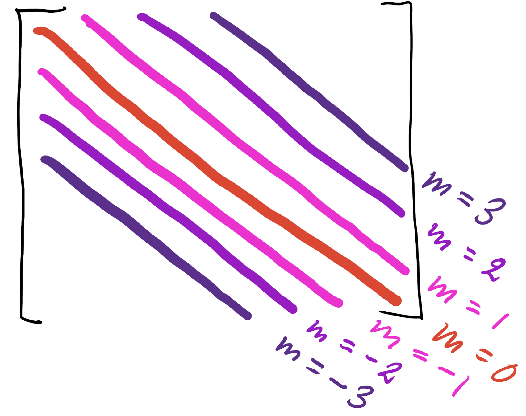
Poisson algebra \( (C^\infty(M),\{\cdot,\cdot\})\) \(\iff\) matrix algebra \( (\mathfrak{u}(n),\frac{1}{\hbar}[\cdot,\cdot])\)

C^\infty(M)\ni \omega \mapsto \mathcal Q_n(f) \in \mathfrak{u}(n)

Quantization map:

1/\sqrt{n^2-1}
\dot\omega + \{\omega,\psi\}= 0
\dot W + \frac{1}{\hbar}[W,S]= 0
\to

Euler equation:

Euler–Zeitlin equation:

Matrix Approach

by Zeitlin

Poisson algebra \( (C^\infty(M),\{\cdot,\cdot\})\) \(\iff\) matrix algebra \( (\mathfrak{u}(n),\frac{1}{\hbar}[\cdot,\cdot])\)

C^\infty(M)\ni \omega \mapsto \mathcal Q_n(f) \in \mathfrak{u}(n)

Quantization map:

Matrix Approach

by Zeitlin

Poisson algebra \( (C^\infty(M),\{\cdot,\cdot\})\) \(\iff\) matrix algebra \( (\mathfrak{u}(n),\frac{1}{\hbar}[\cdot,\cdot])\)

C^\infty(M)\ni \omega \mapsto \mathcal Q_n(f) \in \mathfrak{u}(n)

Quantization map:

Zeitlin Model on the Sphere

\displaystyle \dot W + \frac{1}{\hbar}[W,S] = 0
\quad -\Delta_n S = W

Hoppe–Yau Laplacian

\Delta_n S = \frac{1}{\hbar^2}\sum_{\alpha=1}^3 [[S, X_\alpha], X_\alpha]
\Delta_n T_{\ell,m} = -\ell(\ell+1)T_{\ell,m}

Geometric Properties

\displaystyle \dot W + \mathrm{ad}^*_{\mathrm d H(W)} W = 0

symplectic leaf =

coadjoint orbit =

isospectral surface

W

Lie-Poisson system on \(\mathfrak{su}(n)^*\)

for Hamiltonian

\displaystyle H_n(W) = \frac{2\pi}{n}\operatorname{Tr}(W^\dagger (-\Delta_n)^{-1}W)

Casimir functions

\displaystyle C_{n,f}(W) = \frac{4\pi}{n}\operatorname{Tr}(f(\mathrm iW))

Criticism

  • From numerical community
    low order of convergence

     
  • From fluid community
    enstrophy should dissipate
    (forward cascade in 2-D turbulence)

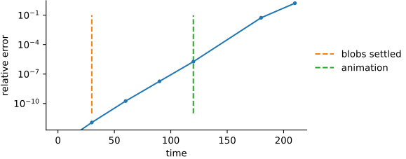
Long Time Accuracy is Impossible

Convergence, matrix hydrodynamics: [Gallagher 2002, M. & Viviani 2026]

Convergence, spectral methods: [e.g. Bardos & Tadmor 2015]

\lVert \tilde\omega_t^n - \omega_t \rVert_{H^{-1}} \lesssim \mathrm e^{2t \lVert \omega_0 \rVert_{L^\infty}}\left(n^{-2(s+1)}\lVert \omega_0\rVert_{H^{s}} + n^{1-s} \max_{\tau\leq t}\lVert \omega_\tau\rVert_{H^{s}} \right) % s' = s-1 -> s = s'+1, s>2 -> s'>1

gives order \(p = (s-1)/2\)

\(\lVert \omega_t \rVert_{C^1} \lesssim \mathrm e^{\mathrm e^{c t}} \)

\lVert \tilde\omega_t^n - \omega_t \rVert_{L^2} \lesssim n^{-1}\left( \ldots \right)\mathrm{exp}\left(\int_0^t (\ldots + \lVert \nabla\omega_\tau\rVert_{L^\infty})\mathrm d \tau \right) % s' = s-1 -> s = s'+1, s>2 -> s'>1

short

time

long

time

Long Time Accuracy is Impossible

Convergence, matrix hydrodynamics: [Gallagher 2002, M. & Viviani 2026]

Convergence, spectral methods: [e.g. Bardos & Tadmor 2015]

\lVert \tilde\omega_t^n - \omega_t \rVert_{H^{-1}} \lesssim \mathrm e^{2t \lVert \omega_0 \rVert_{L^\infty}}\left(n^{-2(s+1)}\lVert \omega_0\rVert_{H^{s}} + n^{1-s} \max_{\tau\leq t}\lVert \omega_\tau\rVert_{H^{s}} \right) % s' = s-1 -> s = s'+1, s>2 -> s'>1

gives order \(p = (s-1)/2\)

\(\lVert \omega_t \rVert_{C^1} \lesssim \mathrm e^{\mathrm e^{c t}} \)

\lVert \tilde\omega_t^n - \omega_t \rVert_{L^2} \lesssim n^{-1}\left( \ldots \right)\mathrm{exp}\left(\int_0^t (\ldots + \lVert \nabla\omega_\tau\rVert_{L^\infty})\mathrm d \tau \right) % s' = s-1 -> s = s'+1, s>2 -> s'>1

short

time

long

time

Long Time Accuracy is Impossible

Convergence, matrix hydrodynamics: [Gallagher 2002, M. & Viviani 2026]

Convergence, spectral methods: [e.g. Bardos & Tadmor 2015]

\lVert \tilde\omega_t^n - \omega_t \rVert_{H^{-1}} \lesssim \mathrm e^{2t \lVert \omega_0 \rVert_{L^\infty}}\left(n^{-2(s+1)}\lVert \omega_0\rVert_{H^{s}} + n^{1-s} \max_{\tau\leq t}\lVert \omega_\tau\rVert_{H^{s}} \right) % s' = s-1 -> s = s'+1, s>2 -> s'>1

gives order \(p = (s-1)/2\)

\(\lVert \omega_t \rVert_{C^1} \lesssim \mathrm e^{\mathrm e^{c t}} \)

\lVert \tilde\omega_t^n - \omega_t \rVert_{L^2} \lesssim n^{-1}\left( \ldots \right)\mathrm{exp}\left(\int_0^t (\ldots + \lVert \nabla\omega_\tau\rVert_{L^\infty})\mathrm d \tau \right) % s' = s-1 -> s = s'+1, s>2 -> s'>1

short

time

long

time

Long Time Accuracy is Impossible

Convergence, matrix hydrodynamics: [Gallagher 2002, M. & Viviani 2026]

Convergence, spectral methods: [e.g. Bardos & Tadmor 2015]

\lVert \tilde\omega_t^n - \omega_t \rVert_{H^{-1}} \lesssim \mathrm e^{2t \lVert \omega_0 \rVert_{L^\infty}}\left(n^{-2(s+1)}\lVert \omega_0\rVert_{H^{s}} + n^{1-s} \max_{\tau\leq t}\lVert \omega_\tau\rVert_{H^{s}} \right) % s' = s-1 -> s = s'+1, s>2 -> s'>1

gives order \(p = (s-1)/2\)

\(\lVert \omega_t \rVert_{C^1} \lesssim \mathrm e^{\mathrm e^{c t}} \)

\lVert \tilde\omega_t^n - \omega_t \rVert_{L^2} \lesssim n^{-1}\left( \ldots \right)\mathrm{exp}\left(\int_0^t (\ldots + \lVert \nabla\omega_\tau\rVert_{L^\infty})\mathrm d \tau \right) % s' = s-1 -> s = s'+1, s>2 -> s'>1

short

time

long

time

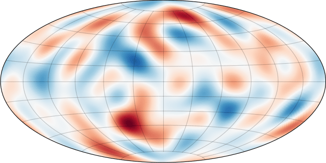
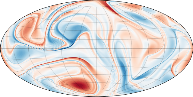
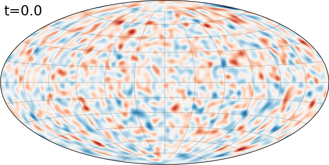
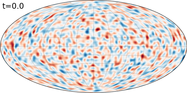
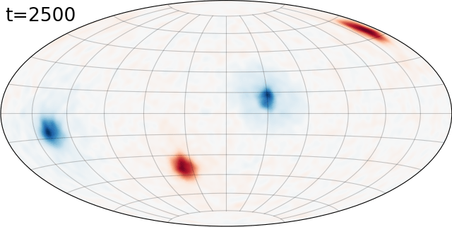
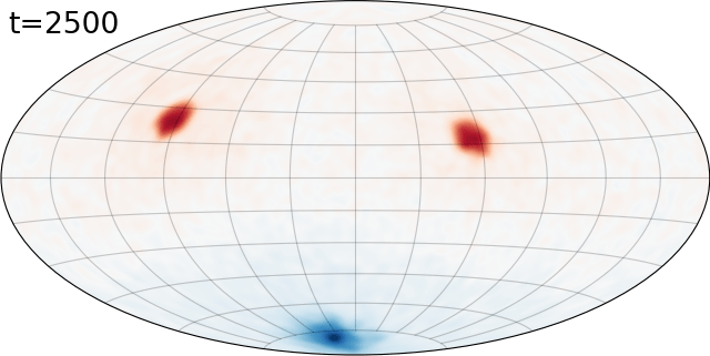
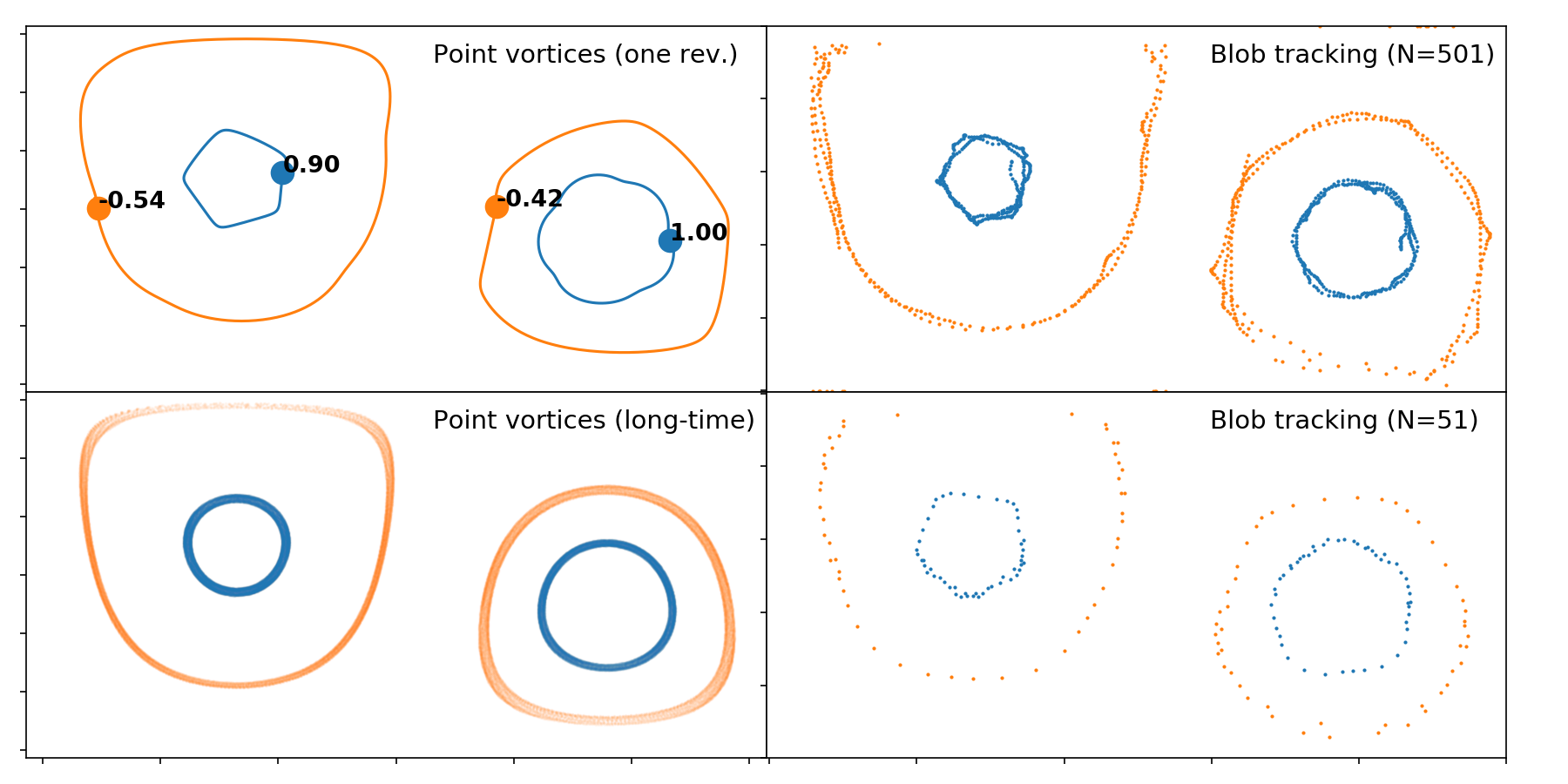
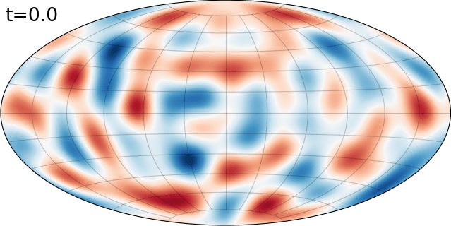
Example: Vortex Condensation as Statistical Behavior

Vortex condensation:

L = 0
L \approx 1

Example: Vortex Condensation as Statistical Behavior

Vortex condensation:

L = 0
L \approx 1

Example: Vortex Condensation as Statistical Behavior

Vortex condensation:

L = 0
L \approx 1

Example: Vortex Condensation as Statistical Behavior

Vortex condensation:

L = 0
L \approx 1

Example: Vortex Condensation as Statistical Behavior

Vortex condensation:

L = 0
L \approx 1

Example: Vortex Condensation as Statistical Behavior

Vortex condensation:

Reversibility:

L = 0
L \approx 1

Example: Vortex Condensation as Statistical Behavior

Vortex condensation:

Reversibility:

L = 0
L \approx 1

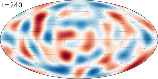
Example: Vortex Condensation as Statistical Behavior

Reversibility:

Lie Poisson Reduction

\mathrm U(n)
\mathfrak{u}(n)^*
W = \mu(Q,P)
Q
I
P
W
W
\mathfrak{u}(n)^*
T_Q^*\mathrm U(n)

Right invariance:

\(\mathcal H(Q,P) = \mathcal H\big((Q,P)\cdot R\big)\)

\dot Q = \frac{\partial \mathcal H}{\partial P},\; \dot P = -\frac{\partial \mathcal H}{\partial Q}
\dot W = [\mathrm dH(W),W]

isospectral flow

coadjoint

orbits

(for Lie group of unitary matrices)

\mu

ISOSYRK Methods

[Viviani, PhD thesis 2020]

\mathrm U(n)
\mathfrak{u}(n)^*
W = \mu(Q,P)
Q
I
P
W
W
\mathfrak{u}(n)^*
T_Q^*\mathrm U(n)

Butcher tableau SYRK \( (A,b)\)

(Isospectral Symplectic Runge–Kutta)

\dot W = [\underbrace{\mathrm dH(W)}_{f(W)},W]

coadjoint

orbits

(Q_{k+1},P_{k+1}) = \Psi_h^{(A,b)}(Q_{k},P_{k})
W_{k+1} = \Phi_h^{(A,b)}(W_k)
\mu

ISOSYRK Methods

[Viviani, PhD thesis 2020]

\mathrm U(n)
\mathfrak{u}(n)^*
W = \mu(Q,P)
Q
I
P
W
W
\mathfrak{u}(n)^*
T_Q^*\mathrm U(n)

Thm [M. & Viviani, 2020] ISOSYRK methods are

  • isospectral
  • symplectic on each coadjoint orbit
    (= isospectral surface)

(Isospectral Symplectic Runge–Kutta)

\dot W = [\underbrace{\mathrm dH(W)}_{f(W)},W]

coadjoint

orbits

ISOSYRK Methods

[Viviani, PhD thesis 2020]

\mathrm U(n)
\mathfrak{u}(n)^*
W = \mu(Q,P)
Q
I
P
W
W
\mathfrak{u}(n)^*
T_Q^*\mathrm U(n)

Example: isospectral mid-point method (ISOMP)

(Isospectral Symplectic Runge–Kutta)

\dot W = [\underbrace{\mathrm dH(W)}_{f(W)},W]

coadjoint

orbits

W_k = \left(I - \frac{h}{2}f(\tilde W) \right)\tilde W \left(I + \frac{h}{2}f(\tilde W) \right)
W_{k+1}= W_k + h[f(\tilde W),\tilde W]

BEA for ISOSYRK Methods

[with E. Bronasco]

\mathrm U(n)
\mathfrak{u}(n)^*
W = \mu(Q,P)
Q
I
P
W
W
\mathfrak{u}(n)^*
T_Q^*\mathrm U(n)

coadjoint

orbits

(Backward Error Analysis)

\psi^*
T^*\mathcal T \simeq \mathcal T^2
\mathcal{BF}

BEA for ISOSYRK Methods

[with E. Bronasco]

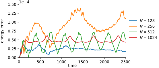
\displaystyle \dot W + \frac{1}{\hbar}[W,S] = 0, \quad -\Delta_n S = W

ISOMP:

Modified Hamiltonian:

h.o.t.

Recall: \(\hbar = \frac{2}{\sqrt{n^2-1}}\)

\textstyle W_k = \big(I - \frac{h}{2\hbar }\tilde S \big)\tilde W \big(I + \frac{h}{2\hbar}\tilde S \big)
\textstyle W_{k+1}= W_k + \frac{h}{\hbar}[\tilde S,\tilde W]

BEA for ISOSYRK Methods

[with E. Bronasco]

\displaystyle \dot W + \frac{1}{\hbar}[W,S] = 0, \quad -\Delta_n S = W

ISOMP:

Modified Hamiltonian:

Recall: \(\hbar = \frac{2}{\sqrt{n^2-1}}\)

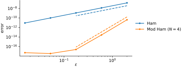
\textstyle \tilde H_{n,h}(W) = H_n(W) - \frac{\epsilon^2}{12}\langle SWS^\dagger, S\rangle +
\textstyle + \frac{\epsilon^2}{24}\langle [S,W],\Delta_n^{-1}[S,W]\rangle + \mathcal O(\epsilon^4)
\textstyle W_k = \big(I - \frac{\epsilon}{2}\tilde S \big)\tilde W \big(I + \frac{\epsilon}{2}\tilde S \big)
\textstyle W_{k+1}= W_k + \epsilon[\tilde S,\tilde W]

Choose \(h = \epsilon\hbar\)

BEA for ISOSYRK Methods

[with E. Bronasco]

\displaystyle \dot W + \frac{1}{\hbar}[W,S] = 0, \quad -\Delta_n S = W
\textstyle \tilde H_{n,h}(W) = H_n(W) - \frac{\epsilon^2}{12}\langle SWS^\dagger, S\rangle +
\textstyle + \frac{\epsilon^2}{24}\langle [S,W],\Delta_n^{-1}[S,W]\rangle + \mathcal O(\epsilon^4)

BEA for ISOSYRK Methods

[with E. Bronasco]

\displaystyle \dot W + \frac{1}{\hbar}[W,S] = 0, \quad -\Delta_n S = W

Thm [Bronasco & M 2026]:

  • \(\omega_0\in C^\infty(\mathbb S^2)\) and \(W_0 = \mathcal Q_n(\omega_0)\)
  • ISOSYRK \(W_{k}\mapsto W_{k+1}\) with \(h = \epsilon \hbar = \frac{2\epsilon }{\sqrt{n^2-1}}\)
|\tilde H_{n,h}^N(W_k)- \tilde H_{n,h}^N(W_0)| \leq 2\pi A(\lVert \omega_0\rVert_{L^\infty}) \mathrm e^{-\epsilon_0/(2\epsilon\lVert \omega_0\rVert_{L^\infty})}

for \(t_k = hk \leq \mathrm e^{-\epsilon_0/(2\epsilon\lVert \omega_0\rVert_{L^\infty})}\)

  • \( A(r) = 2e(1+ 6e C_a)(1+3 e C_a+ 18 C_a r)r^2\)
  • \(\epsilon_0 = 1/(18eC_a)\)

BEA for ISOSYRK Methods

[with E. Bronasco]

\displaystyle \dot W + \frac{1}{\hbar}[W,S] = 0, \quad -\Delta_n S = W
  • Zeitlin, Finite-mode analogs of 2D ideal hydrodynamics
    Phys. D, 1991
  • Hoppe & Yau, Some properties of matrix harmonics on \(S^2\)
    Comm. Math. Phys., 1998
  • M. & Viviani, Two-dimensional fluids via matrix hydrodynamics
    Arch. Ration. Mech. Anal., 2026
  • Bronasco & M., Backward error analysis for matrix discretizations
    of 2-D Euler equations, arXiv:2607:09549

Matrix Hydrodynamics Wants You

!

What is Matrix Hydrodynamics?

By Klas Modin

What is Matrix Hydrodynamics?

Presentation given at the FoCM conference in Vienna, July 2026.
  • 2