


Leonardo Petrini
PhD Student @ Physics of Complex Systems Lab, EPFL Lausanne
Candidate: Leonardo Petrini
Exam jury:
President: Dr. Marcia T. Portella Oberli
Expert: Prof. Lenka Zdeborova
Thesis advisor: Prof. Matthieu Wyart
October 27, 2020
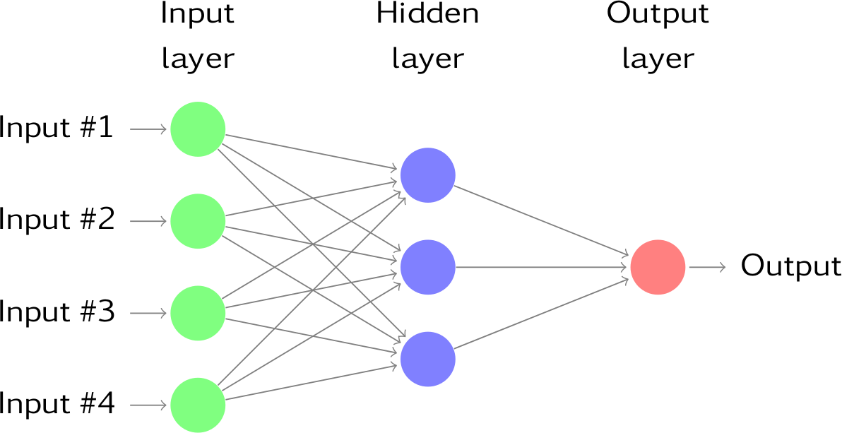
Neural nets are a \(-\) biologically inspired and incredibly effective \(-\) way of parametrizing the function \(f_\theta(\mathbf x)\):
Setting: we have some data observations \(\{\mathbf x^\mu, y^\mu\}_{\mu = 1}^p\) and we suppose there exists an underlying true function \(f^*\) that generated them:
$$y^\mu = f^*(\mathbf x^\mu) + \text{noise}$$
Goal (supervised-learning): find a parametrized function \(f_\theta\) that can properly approximate \(f^*\) and tune the parameters \(\theta\) in order to do so.
Adapted from Geiger et al. (2018)
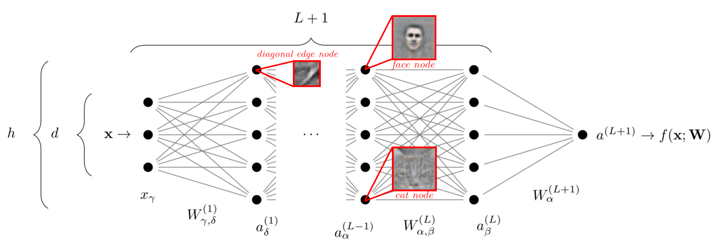
The success of neural nets is often attributed to their ability to
[Mallat (2016)]
e.g. pixels in the corner are unrelated to the class label
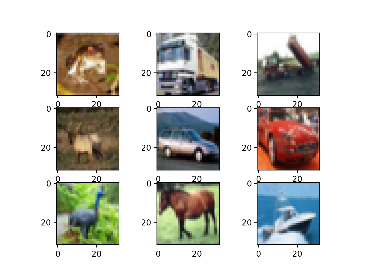
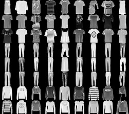
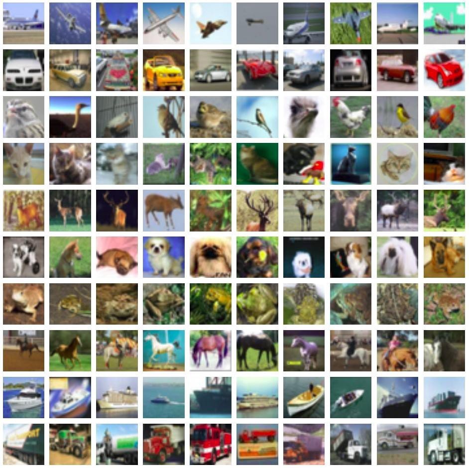
CIFAR10 data-point
or even the
background color
(1) Information-theoretical point of view:
[Shwartz-Ziv and Tishby (2017)]
[Ansuini et al. (2019),
Recanatesi et al. (2019)]
(2) "Geometrical" point of view:
example
starting from [Jacot et al. 2018]...
Lazy Regime
Feature Regime
\(t\): training time
tangent space
tangent space
Lazy Regime
Feature Regime
Jacot et al. (2018): to each net we can associate a kernel, the Neural Tangent Kernel (NTK):
\(t\): training time
tangent space
tangent space
\(\dot \theta = -\nabla_\theta \mathcal{L}\)
Gradient Flow
(weights space)
NTK:
Gradient Flow
in function space
}
NTK
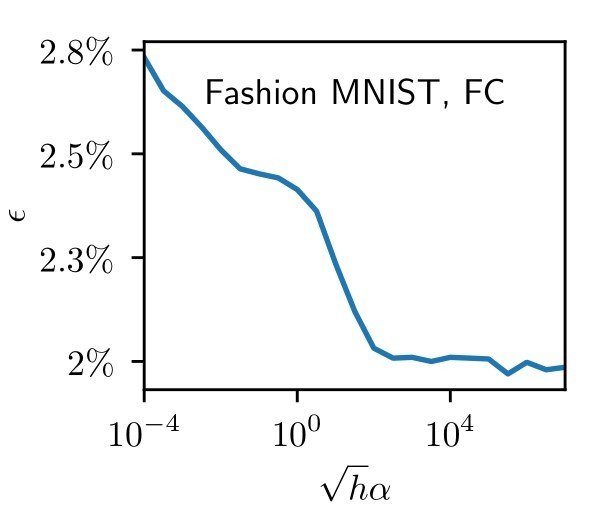
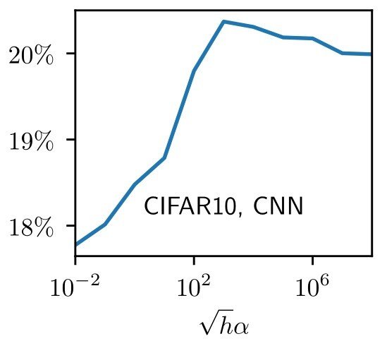
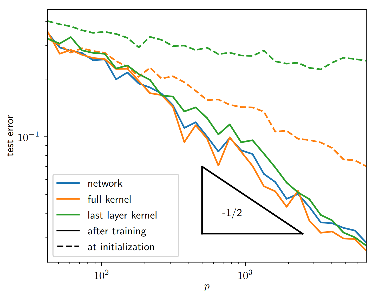
How does operating in the feature or lazy regime affect deep nets performance?
Each regime can be favoured by different architectures and data structures [Geiger et al. 2019]:
Test error
feature lazy
Test error
feature lazy
MNIST, CNN
\(\epsilon_t\)
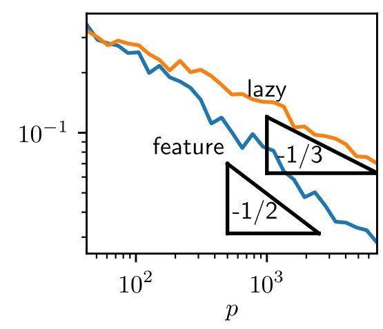
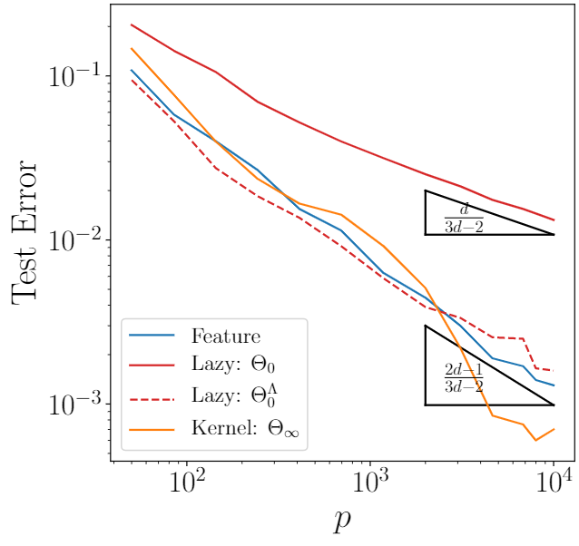
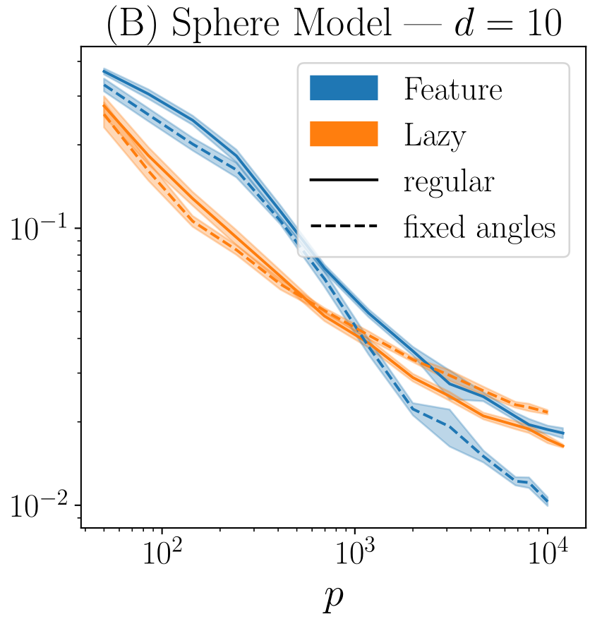
Moreover, if we look at learning curves:
we measure a different exponent \(\beta\) for the two regimes.
In the following, we will use \(\beta\) to characterize performance.
test error
train. set size
To sum up:
Some questions arise:
Part II | the drawbacks:
Part I | the perks:
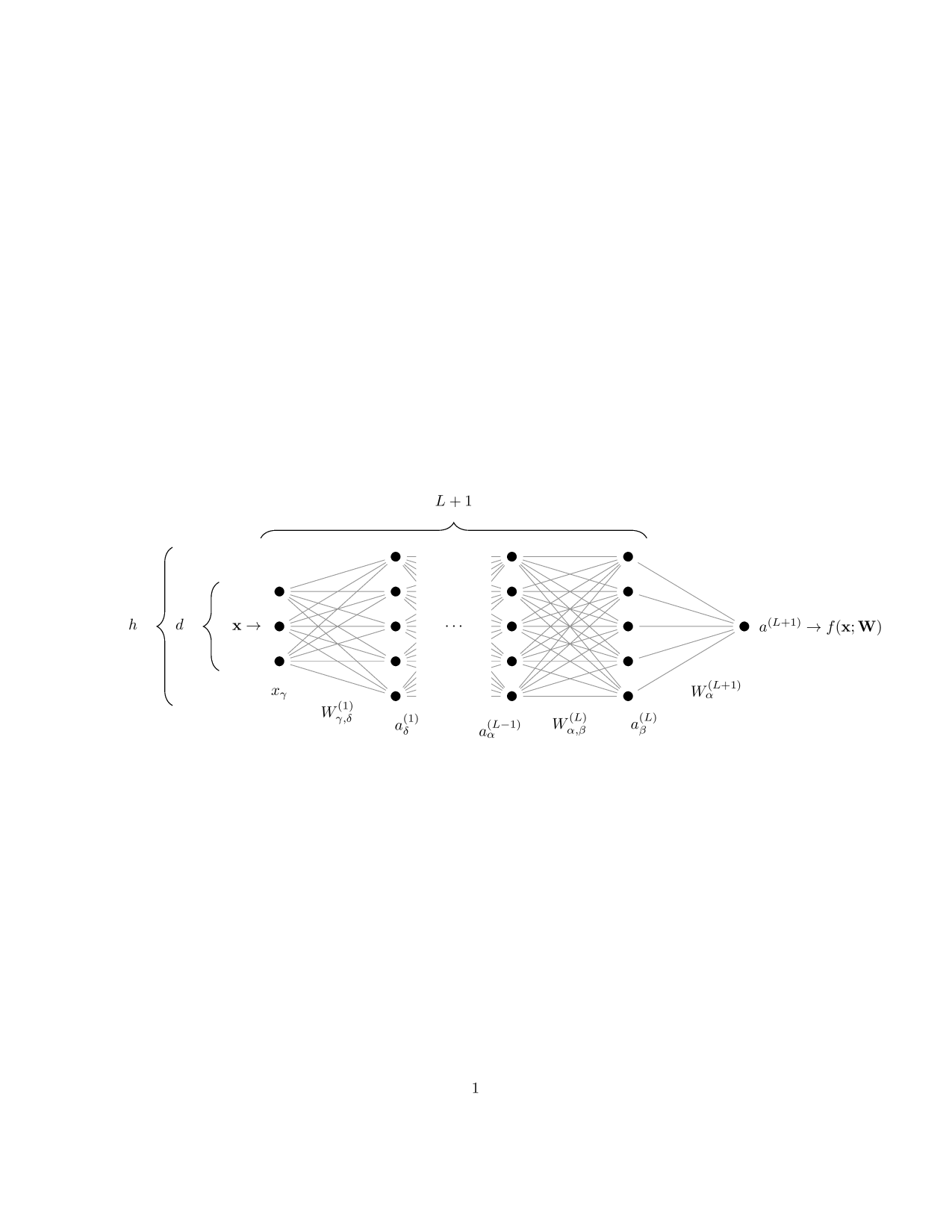
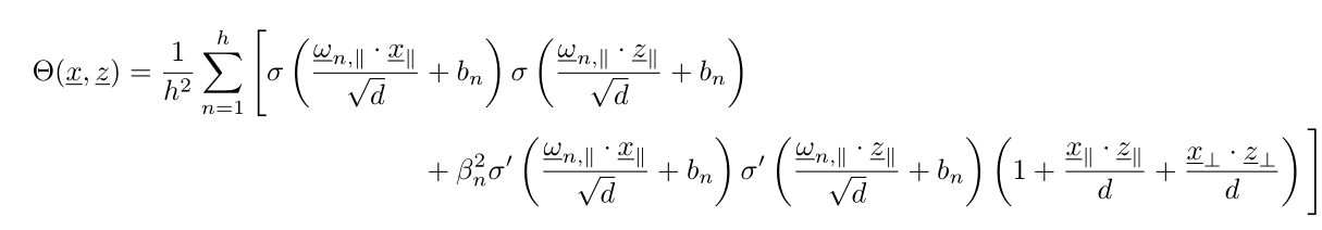
Fully connected one-hidden layer NN:
$$f(\mathbf x) = \frac{1}{h} \sum_{n=1}^h \beta_n \: \sigma \left(\frac{\mathbf{\omega}_n \cdot \mathbf x}{\sqrt{d}} + b_n \right)$$
\(\mathbf x^\mu \sim \mathcal{N}(0, I_d)\), for \(\mu=1,\dots,p\)
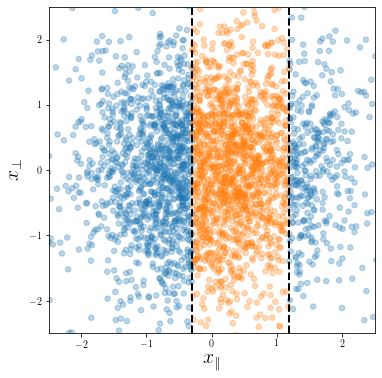
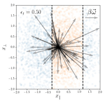
Classification task: \(y(\mathbf x) = y( x_\parallel) \in \{-1, 1\}\)
weights evolution during training
for a subset of neurons
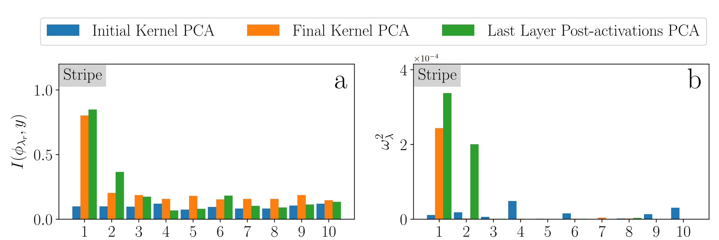
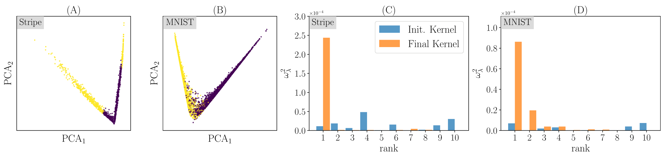
Compression in the feature regime
weights evolution during training
for a subset of neurons
Compression and the Neural Tangent Kernel:
Compression in the feature regime
one-hidden layer fully connected NTK after compressing \(\mathbf x_\bot\)
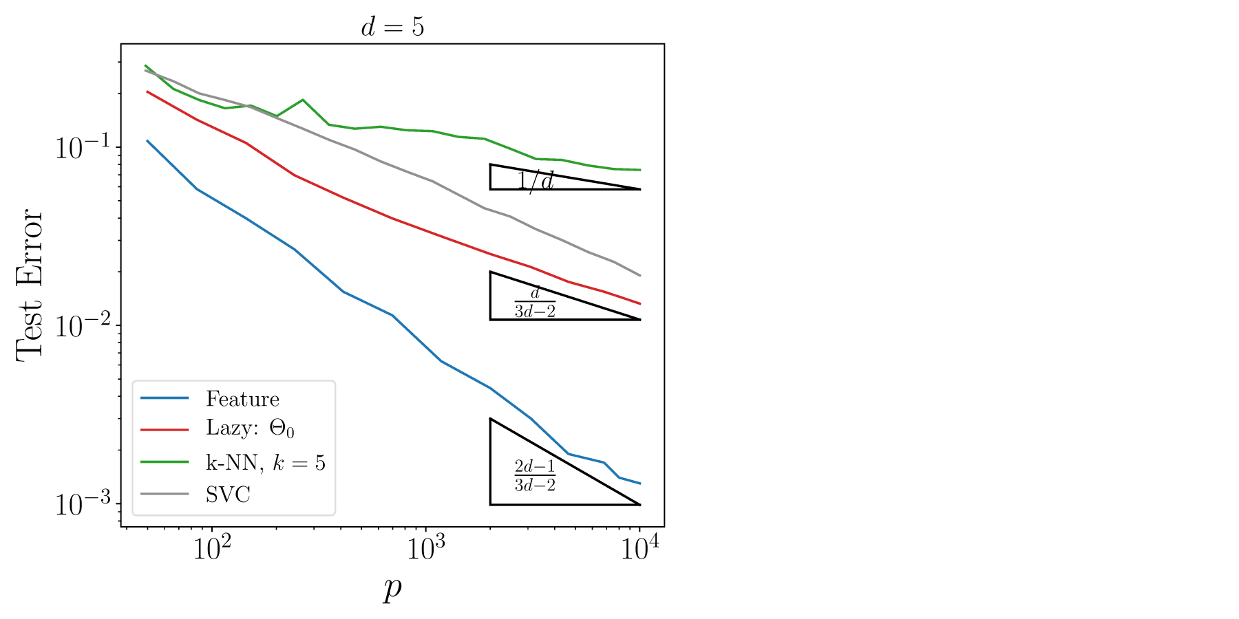
Alignment between kernel eigenvectors and labelling function determines performance (some intuition):
The ideal kernel for a classification target \(y(x)\) would be \(K^*(x, z) = y(x)y(z)\).
A kernel is more performant on a classification target \(y(x)\) the larger is its alignment with the ideal kernel. That is, the larger the overlap between its eigenvectors and \(y(x)\)
Mutual Information
Projection
(training set size)
The kernel at the end of learning performs as good as the network itself!
Compression makes the NTK more performant!
classes interface
o
Support
vectors
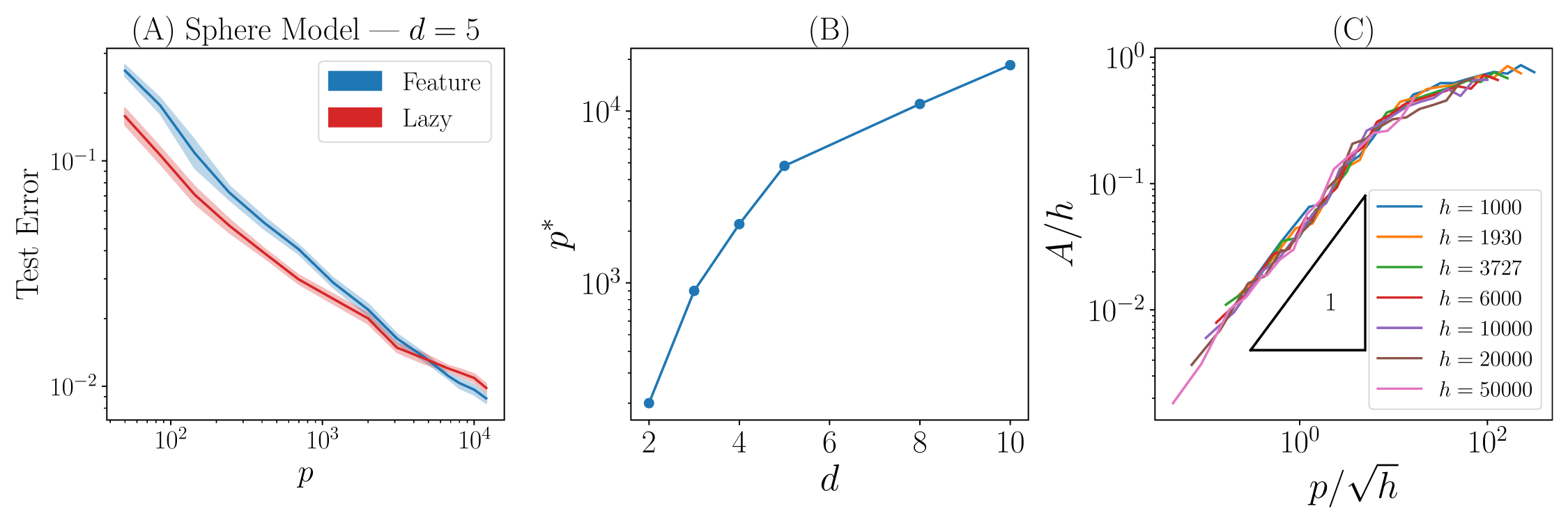
SVs distance suffers the curse of dimensionality but, if the interface is regular enough between two SVs, the curse does not affect kernel performance.
This is only true for classification.
[Paccolat et al. (2020)]
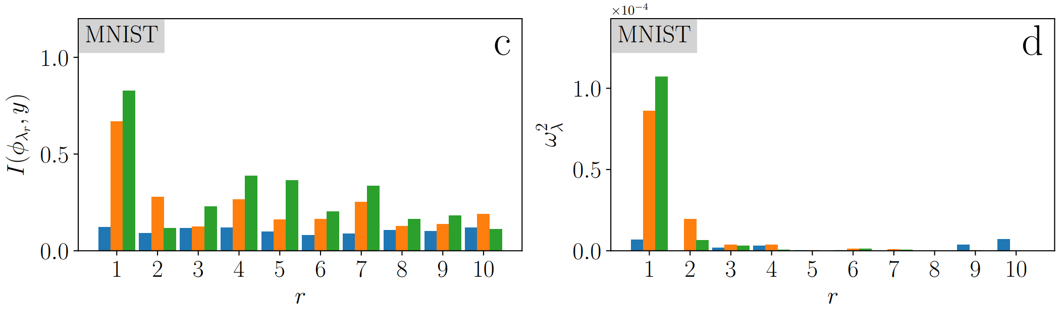
Mutual Information
Projection
Learning Curves
Similarities with Stripe Model
→ hint to compression being key also in MNIST
...
[Ansuini et al. (2019)]
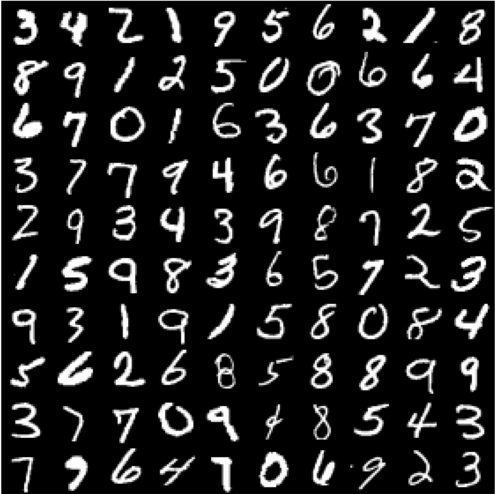
Such a dimension-reduction to a ~1D manifold clearly appears in MNIST as well
Last hidden-layer pre-activations PCA
color: class label
Part II | the drawbacks:
Part I | the perks:
\(\mathbf x^\mu \sim \mathcal{N}(0, I_d)\), for \(\mu=1,\dots,p\)
Classification task is rotationally invariant:
\(y(\mathbf x) = y(||\mathbf {x}||) \in \{-1, 1\}\)
Learning curves | \(d=10\)
\(0\)
e.g. in 1D:
ReLU
\(\mathbf z\)
\(\mathbf x\)
neurons
\(0\)
in 1D:
ReLU
\(\mathbf z\)
\(\mathbf x\)
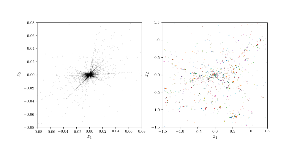
Distribution of \(\mathbf z\) for:
(A) Initialization
(B) Lazy | end of train.
(C) Feature| during tr.
(D) Feature| end of tr.
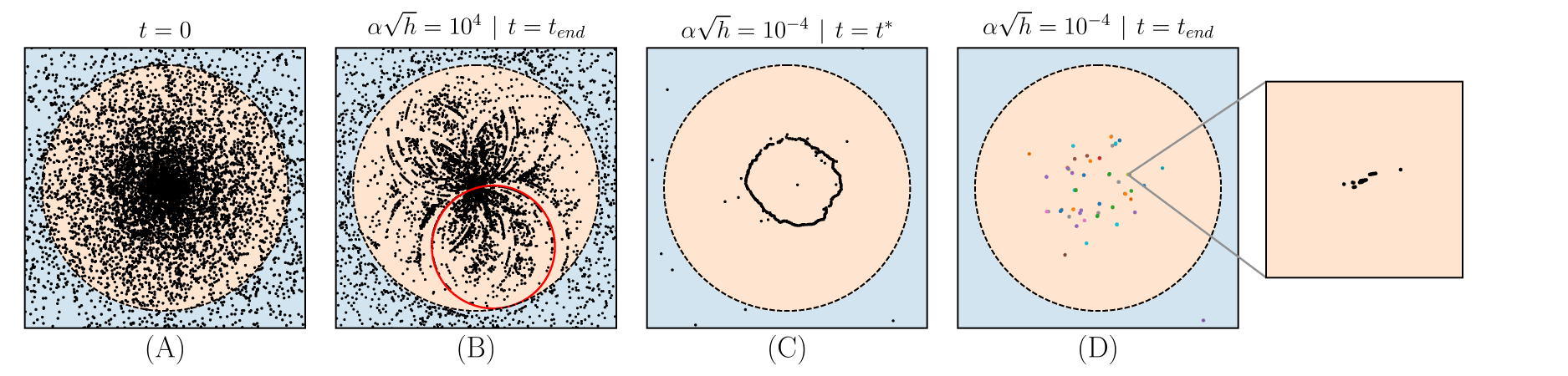
Def. an attractor is a set of neurons that are active on the same subset of training points.
here neurons are grouped together by color, following the attractor definition
Gradient flow dynamics:
$$\dot W = -\nabla_W \mathcal{L}$$
where \(W\) can be any of the net weights \(\omega_n\), \(b_n\), \(\beta_n\).
Recall:
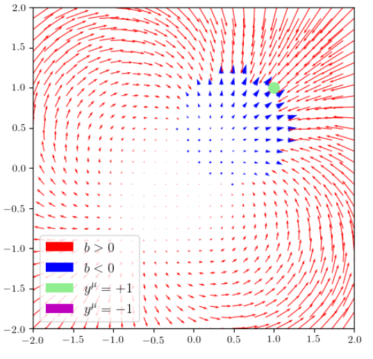
One can derive
the direction of this ineq. depending on the sign of \(b\)
Notice: such an attractor can be replaced by a single neuron without affecting \(f(\mathbf x)\) on the training set.
Short-term goals:
Field \(\dot{\mathbf z}\) for \(p=1\)
Research Goal: extend the study of attractors to other simple models in order to understand how they affect performance and bridge the gap with observations in real data.
10-PCA MNIST | end of train. neurons position
thank you!
Long-term:
By Leonardo Petrini
PhD Candidacy Examination @ Physics Doctoral School, EPFL


