


Leonardo Petrini
PhD Student @ Physics of Complex Systems Lab, EPFL Lausanne
2
1
Leonardo Petrini,* Francesco Cagnetta,* Eric Vanden-Eijnden, Matthieu Wyart
1
1
2
1
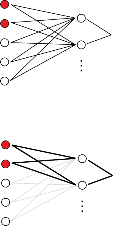
initialization (dense)
trained (sparse)
Geiger et al. (2020a,b); Lee et al. (2020)
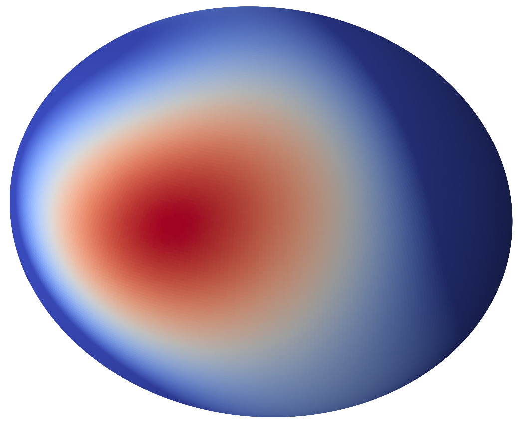
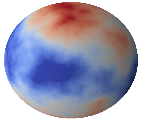
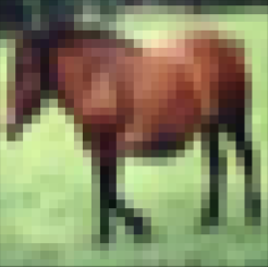
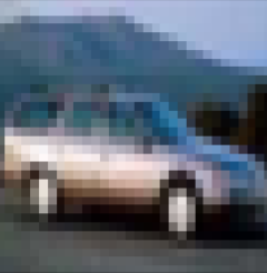
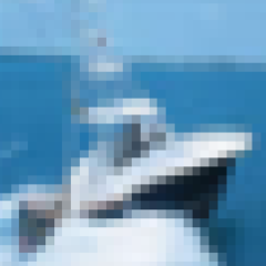
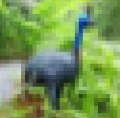
Figure. Kernel predictor is smoother along diffeomorphisms for image classification.
more smooth
Task: regression with \(n\) training points \(\{\bm x\}_{i=1}^n\) uniformly sampled from the hyper-sphere \(\mathbb{S}^{d-1}\) and target function of controlled smoothness \(\nu_t\):
$$\| f^*(\bm{x})-f^*(\bm{y})\| \sim \|\bm{x}-\bm{y}\|^{\nu_t} $$
High smoothness
(large \(\nu_t\))
Low smoothness
(small \(\nu_t\))
log test error
log train set size
log test error
log train set size
feature learning
kernel regime
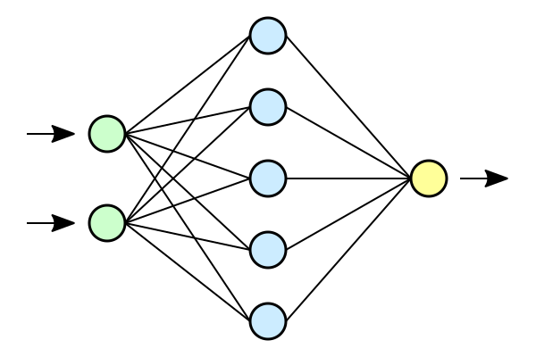
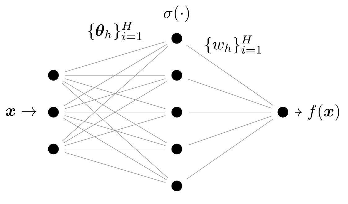
Architecture: one-hidden-layer fully-connected with ReLU activations,$$f(\bm{x}) = \frac{1}{\mathcal{N}} \sum_{h=1}^H w_h \sigma( \bm{\theta}_h\cdot\bm{x}) $$
\(H\to\infty\): the choice of the normalization constant \(\mathcal{N}\) controls the training regime, $$\qquad\qquad\mathcal{N} = H \qquad \qquad \qquad\qquad\qquad\qquad\qquad \mathcal{N} = \sqrt{H}$$
feature learning
kernel regime
Jacot et al. (2018);
Bach (2018); Mei et al. (2018);
Rotskoff, Vanden-Eijnden (2018)...
Architecture: our aim is to approximate the target function by a one-hidden-layer neural network of width \(H\), $$f(\bm{x}) = \frac{1}{\mathcal{N}} \sum_{h=1}^H w_h \sigma( \bm{\theta}_h\cdot\bm{x}) $$
as \(H\to\infty\), the choice of the normalization constant \(\mathcal{N}\) controls the training regime, $$\qquad\qquad\mathcal{N} = H \qquad \qquad \qquad\qquad\qquad\qquad\qquad \mathcal{N} = \sqrt{H}$$
and the predictors take the forms:
feature learning
kernel regime
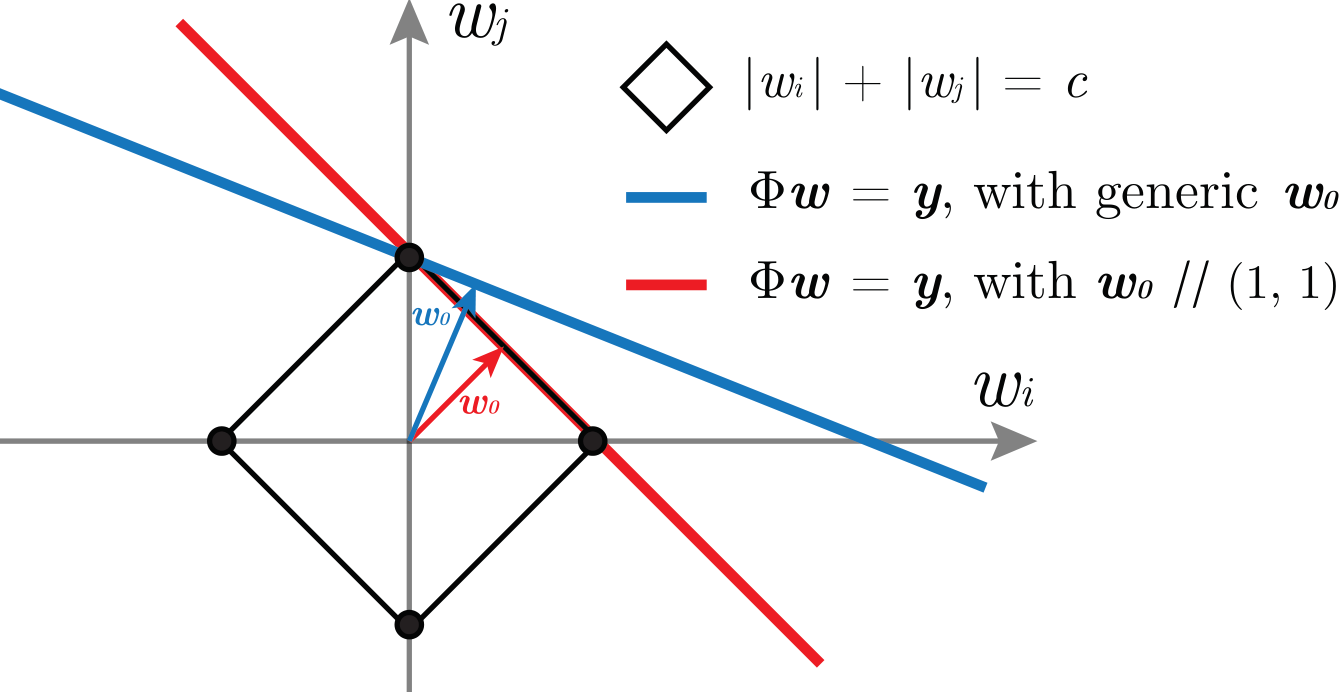
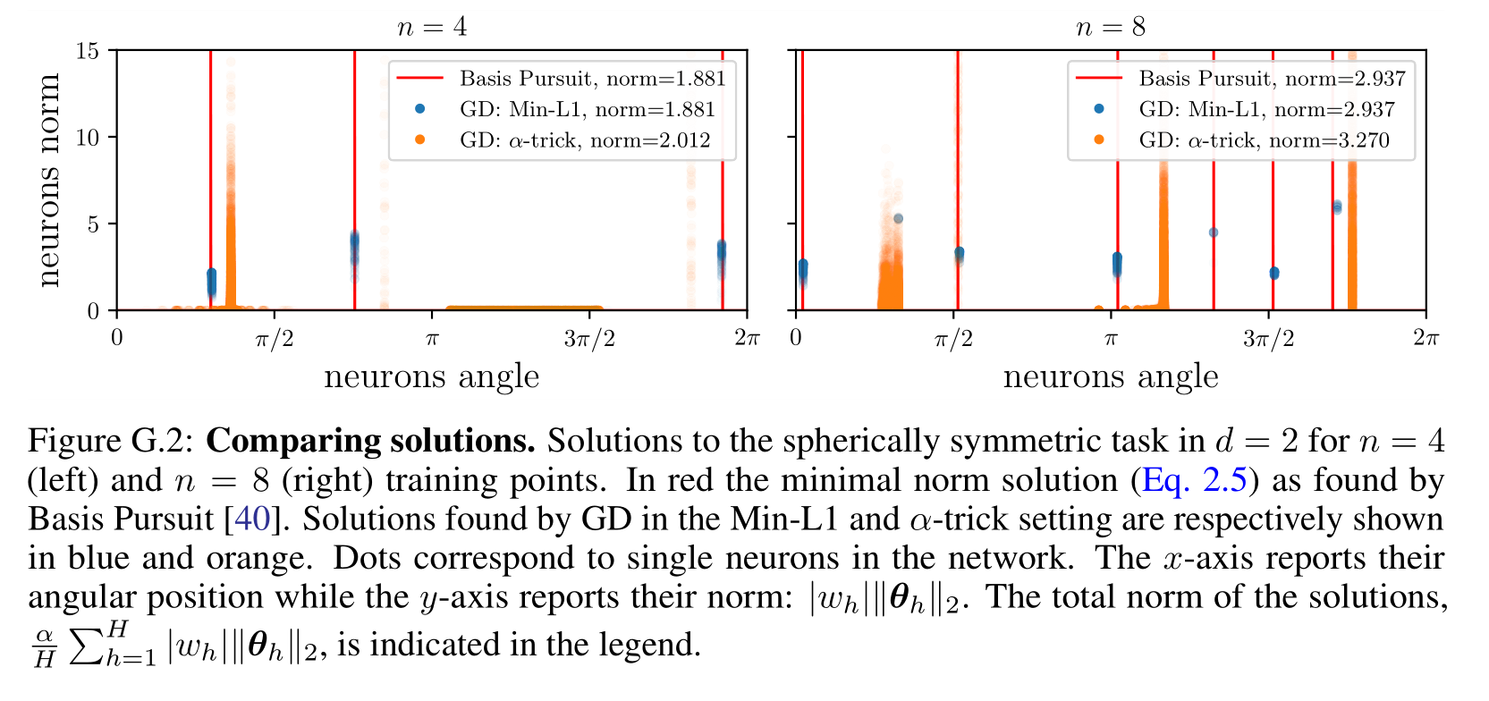
Atomic solution: the feature regime predictor takes the following form,$$f^{\text{FEATURE}}(\bm{x}) = \sum_{i=1}^{n_A} w^*_i \sigma( \bm{\theta}^*_i\cdot\bm{x}) , \quad n_A = O(n),$$
Kernel trick: while the kernel predictor can be written as (with \(K\) the NTK), $$f^{\text{LAZY}}(\bm{x}) =\sum_{i=1}^n g_i K(\bm{x}_i\cdot \bm{x}).$$
Boyer et al. (2019);
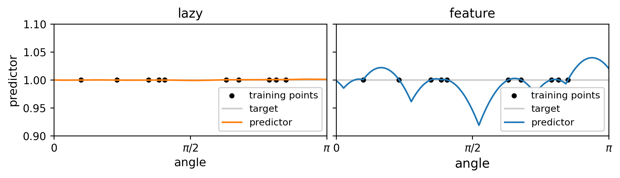
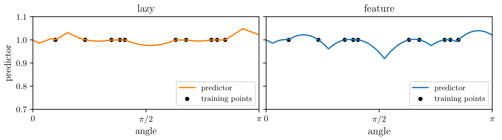
Notice that \(K\) is smoother than the ReLU function \(\sigma\), leading to a smoother predictor.
The scaling of generalization error is controlled by the smoothness of \( \sigma, \, K\):
predictor
target
predictor
training point
Thank you.
end
vs.
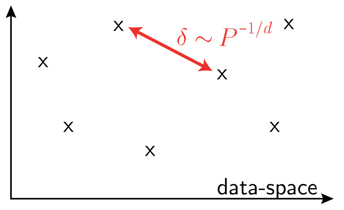
\(P\): training set size
\(d\) data-space dimension
Is the secret of NNs in their ability to capture this structure?
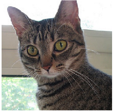
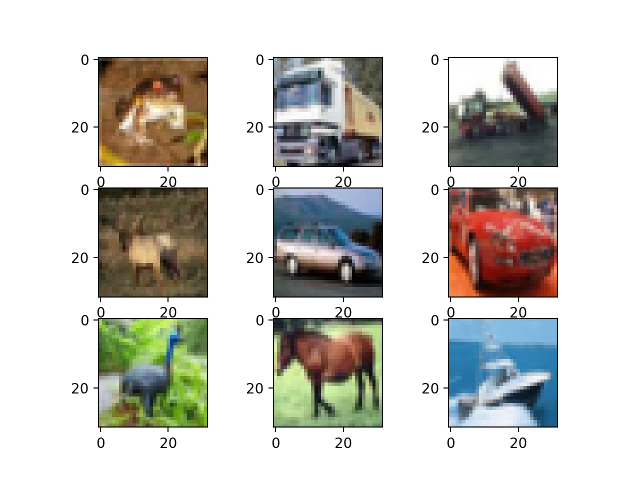
Cat
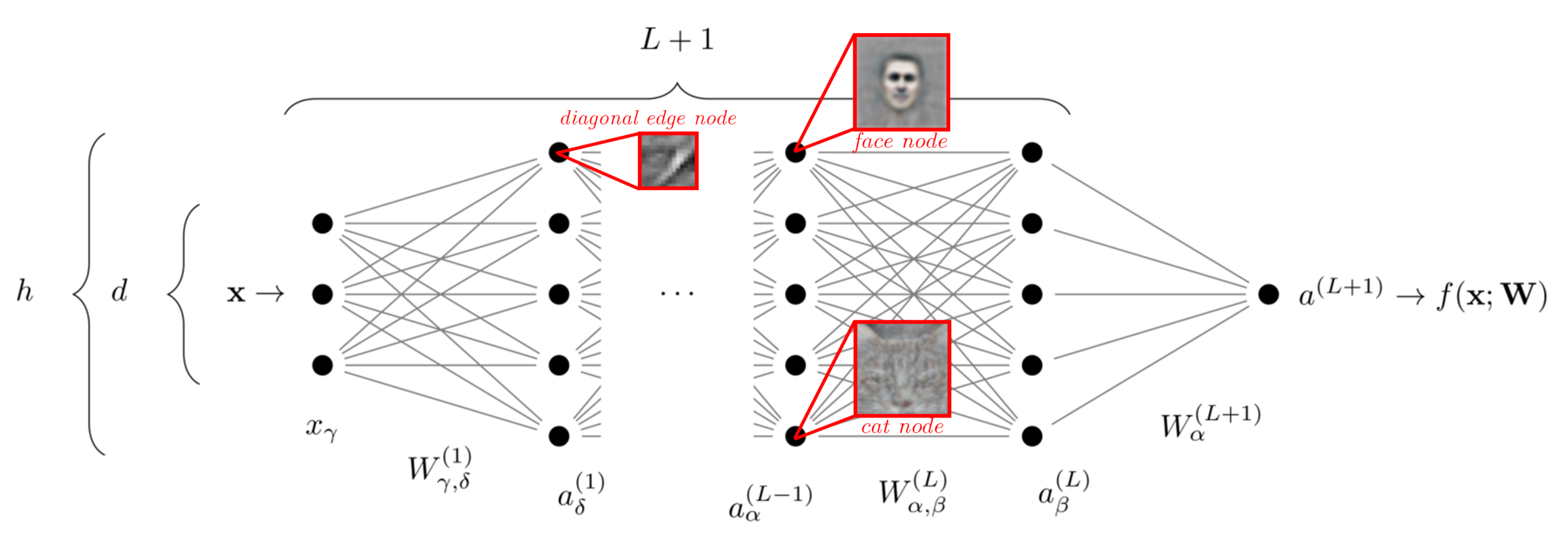
The success of neural nets is often attributed to their ability to learn relevant features of the data
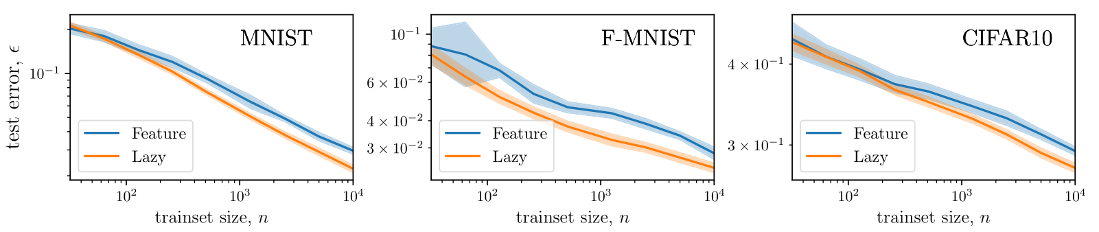
Still, this feature learning is not always beneficial. See for example the training of fully-connected nets on images:
Geiger et al. (2020a,b); Lee et al. (2020)
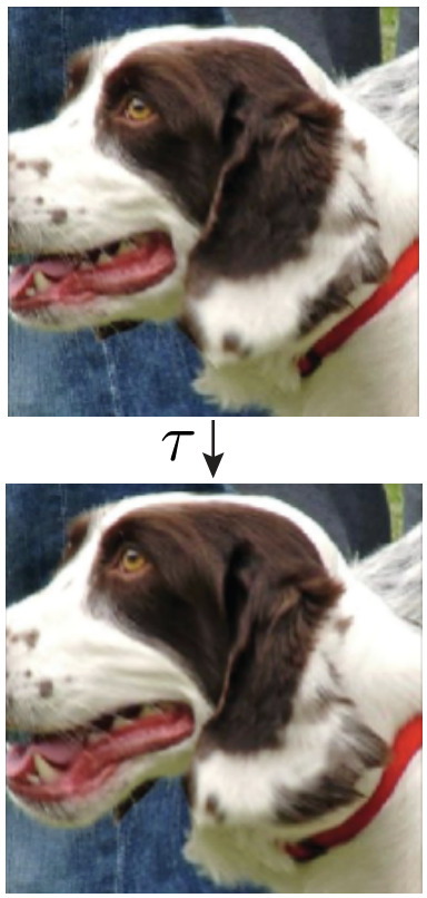
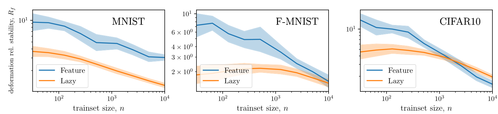
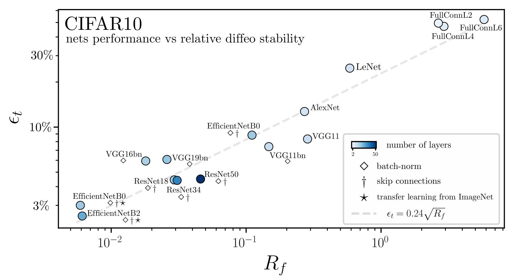
test error
deformation stability
[Petrini et al. 2021]
initialization
FCNs
Moreover, FCNs do not learn a meaningful representation of the data:
Perks and drawbacks of learning features in neural nets?
two training regimes exist, depending on the initialization scale
feature learning
(rich, hydrodynamic...)
neural representation evolves
lazy training
\(\sim\) kernel method
vs.
Jacot et al. (2018); Chizat et al. (2019); Bach (2018); Mei et al. (2018); Rotskoff, Vanden-Eijnden (2018)...
Bach (2017);
Chizat and Bach (2020); Ghorbani et al. (2019, 2020); Paccolat et al. (2020);
Refinetti et al. (2021);
Yehudai, Shamir (2019)...
How to rationalize the feature < lazy case?
e.g.
CIFAR10 data-point
deformation stability
[Petrini et al. 2021]
Task: regression with \(n\) training points \(\{\bm x\}_{i=1}^n\) uniformly sampled from the hyper-sphere \(\mathbb{S}^{d-1}\) and target a Gaussian random process
$$f^*(\bm x) = \sum_{k > 0} \sum_{l=1}^{\mathcal{N_{k, d}}} f_{k, l}^* Y_{k, l}(\bm x) \quad \text{with} \quad \mathbb{E}[{f^*_{k,l}}]=0,\quad \mathbb{E}[{f^*_{k,l}f^*_{k',l'}}] = c_k\delta_{k,k'}\delta_{l, l'},$$
with controlled power spectrum decay
$$c_k\sim k^{-2\nu_t -(d-1)} \quad \text{for}\quad k\gg 1.$$
This determines the target smoothness in real space
$$\mathbb{E}[{\vert f^*(\bm{x})-f^*(\bm{y})\rvert^2}]=O( |\bm{x}-\bm{y}|^{2\nu_t} )=O((1-\bm{x}\cdot\bm{y} )^{\nu_t} ) \quad\text{ as }\ \ \bm{x}\to\bm{y}.$$
spherical
harmonics
We consider a one-hidden-layer ReLU network of width \(H\), $$f^{\xi}_H(\bm{x}) = \frac{1}{H^{1-\xi/2}} \sum_{h=1}^H \left(w_h \sigma( \bm{\theta}_h\cdot\bm{x}) - \xi w_h^0 \sigma(\bm{\theta}_h^0\cdot \bm{x})\right),$$
where \(\xi\) controls the training regime such that we get well-defined \(H \to\infty\) limits:
initialization
features
weights
ReLU
Recall:
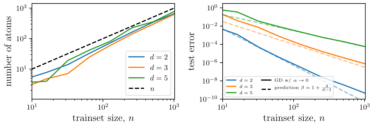
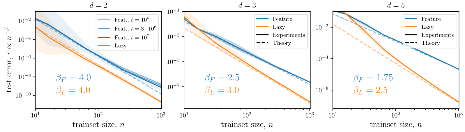
The mean-square error measures the performance in both regimes: $$\epsilon(n) = \mathbb{E}_{f^*} \int_{\mathbb{S}^{d-1}} d\bm x \, ( f^n(\bm{x})-f^*(\bm{x}))^2 = \mathcal{A}_d n^{-\beta} + o(n^{-\beta}),$$ and we are interested in predicting the decay exponent \(\beta\) controlling the behavior at large \(n\). In both regimes, the predictor reads $$f^n(\bm{x}) = \sum_{j=1}^{{O}(n)} g_j \varphi(\bm{x}\cdot\bm{y}_j)\qquad\qquad\qquad\qquad\qquad\qquad\qquad\qquad$$
We first threat \(d=2\) and then generalize to any \(d\).
Recall:
In \(d=2\) (random functions on a circle), we can compute \(\beta\) as \(n\to\infty\) by:
Therefore:
We quantify performance in the two regimes as $$\epsilon(n) = \mathbb{E}_{f^*} \int_{\mathbb{S}^{d-1}} d\bm x \, ( f^n(\bm{x})-f^*(\bm{x}))^2 = \mathcal{A}_d n^{-\beta} + o(n^{-\beta}).$$
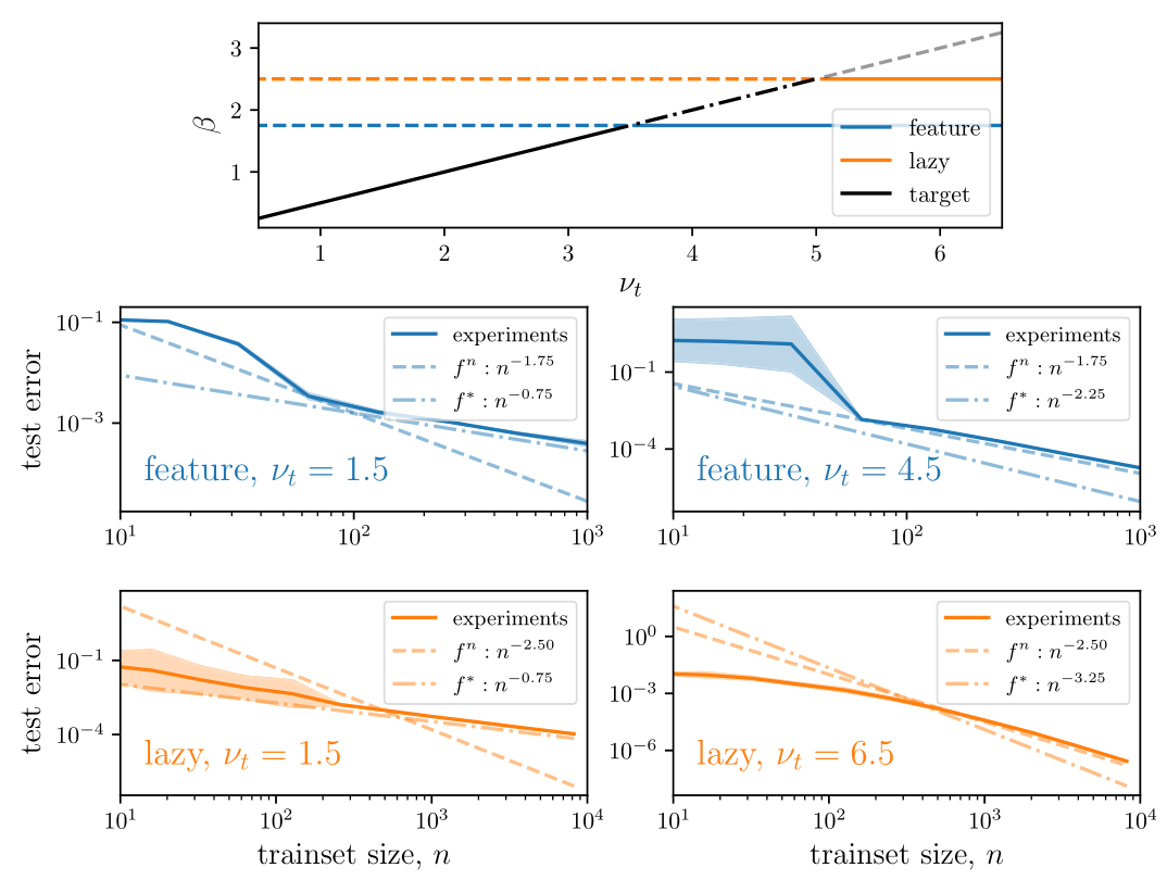
The prediction for \(\beta\) relies on the spectral bias ansatz (S.B.): $$\epsilon(n) \sim \sum_{k\geq k_c} \sum_{l=1}^{\mathcal{N}_{k,d}} (f^n_{k,l}-f^*_{k,l})^2 \sim \sum_{k\geq k_c} \sum_{l=1}^{\mathcal{N}_{k,d}} \mathbb{E}_{f^*}[(g^n_{k,l})^2] \varphi_k^2+ k^{-2\nu_t-(d-1)},$$ were we decomposed the test error into the base of spherical harmonics.
(S.B.): for the first \(n\) modes the predictor coincides with the target function.
To sum up, the predictor in both regimes can be written as $$f^n(\bm{x}) = \sum_{j=1}^{{O}(n)} g_j \varphi(\bm{x}\cdot\bm{y}_j) := \int_{\mathbb{S}^{d-1}} g^n(\bm{y}) \varphi(\bm{x}\cdot\bm{y}) d\bm y,$$ which we then casted as a convolution by introducing \(g^n(\bm{x})=\sum_j |\mathbb{S}^{d-1}|g_j \delta(\bm{x}-\bm{y}_j)\).
We built a theory for the MSE minimizes, do the predictions hold when the network is trained by gradient descent (GD)?
While (1.) effectively recovers the minimal norm solution, (2.) does not. However, we show that (2.) also finds a solution that is sparse and supported on \(n_A \leq n\) neurons.
Chizat et al. (2019)
Jacot et al. (2018)
We show here the agreement between theory and
experiments for a smooth target:
Predictions:
For fully-connected networks
e.g.
Bach (2017);
Chizat and Bach (2020); Ghorbani et al. (2019, 2020); Paccolat et al. (2020);
Refinetti et al. (2021);
Yehudai, Shamir (2019)...
Does (2.) hold for FCNs on image datasets?
We argue that the view proposed also holds for images as:
By Leonardo Petrini


