









Sarah Dean PRO
asst prof in CS at Cornell
CS Colloquium at RPI, September 2026
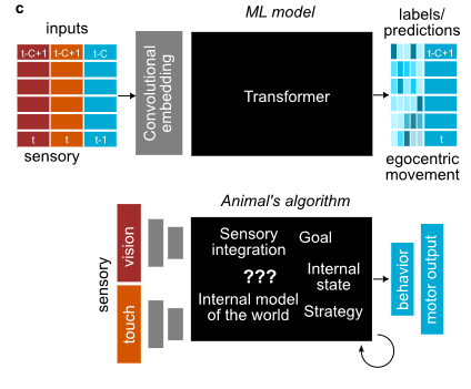
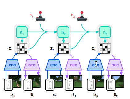
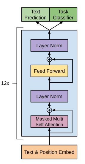
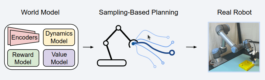
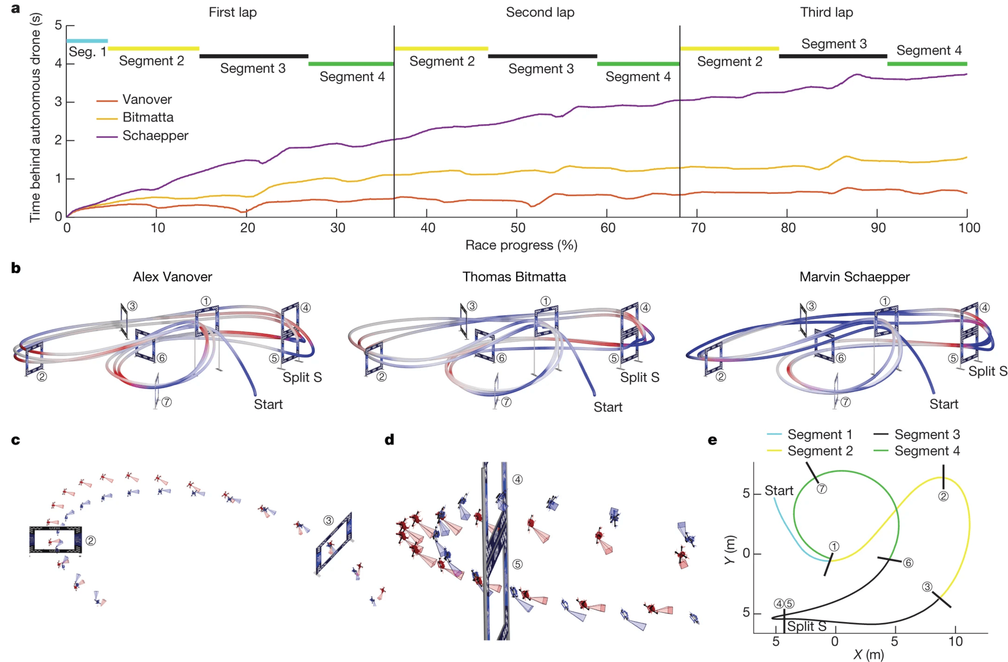
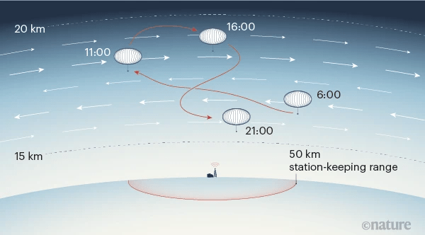
Auto-regressive architectures trained with next element prediction loss have had great success in many domains
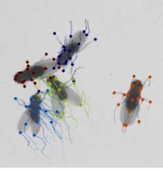
Eyjolfsdottir & Branson, Agent-Centric Animal Pose Forecasting
Haffner et al., Mastering Diverse Domains through World Models
Radford et al., Improving Language Understanding by Generative Pre-Training
natural language
robotics
biology
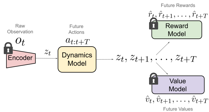
Many researchers are interested in intermediate network activations, whether for use in downstream tasks or for scientific understanding
Levy et al., Simulation Distillation: Pretraining World Models
in Simulation for Rapid Real-World Adaptation
Eyjolfsdottir & Branson, Agent-Centric Animal Pose Forecasting
robotics
biology
filter
controller
\(y\)
\(u\)
system
\(x\)
Partially observed stochastic dynamical system
$$ x_{t+1} = f(x_t,u_t,w_t),\quad y_t = g(x_t, v_t) $$
ex: UAV
\(x\)
\(f\)
\(g\)
\(w\)
\(v\)
Irreducible uncertainty in state is described by the posterior distribution
$$P(x_t | y_0, u_0, y_1, u_1,...,y_t) $$
\(u\)
\(y\)
$$x_0\sim \mathcal D_0, w_t\sim \mathcal D_w, v_t\sim \mathcal D_v$$
Computing this posterior is called filtering $$P(x_t|y_0,...,y_t) \propto P(x_{t-1}|y_0,...,y_{t-1}) P(x_t|x_{t-1} , u_t, y_{t})$$ but for general distributions it can be hard
Setting with no models, only observations
$$ (y_0, u_0, y_1, u_1, \dots, y_T, u_T) $$
ex: UAV
\(x\)
\(?\)
\(?\)
\(w\)
\(v\)
For any similarity transform, \(\tilde x = S(x)\) is an equivalent state space representation with identical input/output behavior
$$ \tilde f = S \circ f \circ S^{-1}, \qquad \tilde g = g \circ S^{-1} $$
\(u\)
\(y\)
future
\(h_t \approx x_t??\)
past
\(\exists S ~\text{s.t.}~ S(h_t)\approx \arg\max_{x_t} P(x_t|\text{past})??\)
posterior?
\(h_t \approx \arg\max_{x_t} P(x_t|\text{past})??\)
posterior, up to similarity
transform?
ex: UAV
Kinematic equations:
\(f_t = m a_t\)
\(v_{t+1} = v_t + a_t\)
\(p_{t+1} = p_t + v_t\)
\( \begin{bmatrix}p_{t+1}\\ v_{t+1} \end{bmatrix} = \begin{bmatrix} 1 & 1\\ 0 & 1\end{bmatrix} \begin{bmatrix}p_t\\ v_t\end{bmatrix} + \begin{bmatrix}0\\ 1/m\end{bmatrix}f_t\)
\((u_t+w_t)\)
\(y_t = \begin{bmatrix} 1 & 0 \end{bmatrix} x_t + v_t\)
\(=: x_t\)
Consider linear dynamics and measurement functions: $$ x_{t+1} = A x_t + B u_t + w_t, \qquad y_t = C x_t + v_t $$
Guassian initial state and noise: $$x_0\sim \mathcal N(0,\Sigma_0), \quad w_t\sim\mathcal N(0,\Sigma_w),\quad v_t\sim \mathcal N(0,\Sigma_v)$$
\(x\)
\(A, B\)
\(C\)
\(w\)
\(v\)
\(u\)
\(y\)
For linear-Gaussian systems, efficient posterior computation via Kalman filter:
We have that \(P(x_t \mid y_{0:t-1}, u_{0:t-1})\) = \(\mathcal N(\hat x_{t}, \Sigma_{t})\)
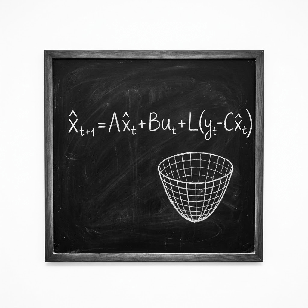
Quickly converges to steady-state Kalman filter (SS-KF) where \(\Sigma_t=\Sigma\) and \(L_t=L\)
does not depend on inputs or outputs
mean/mode
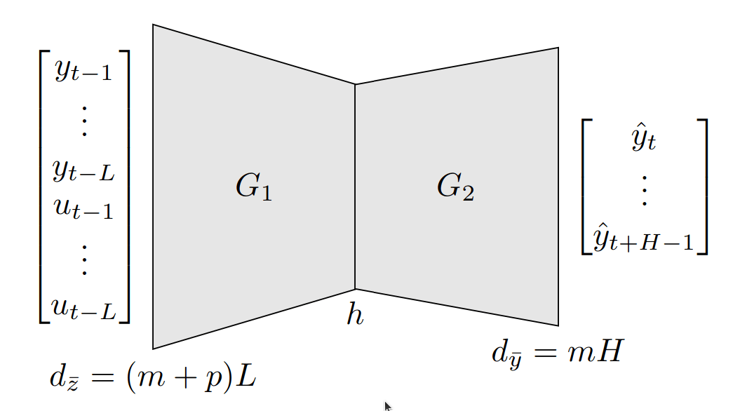
Idea: train an auto-regressive model on \((y_0, u_0, y_1, u_1, \dots, y_T, u_T)\)
\(L\) past inputs/outputs
\(H\) future outputs
two layer linear network
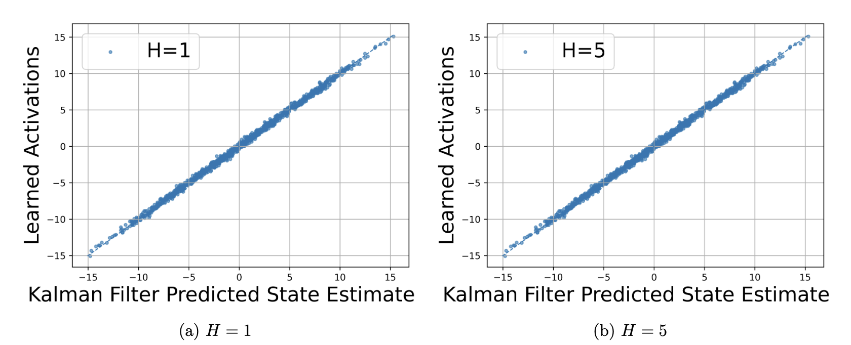
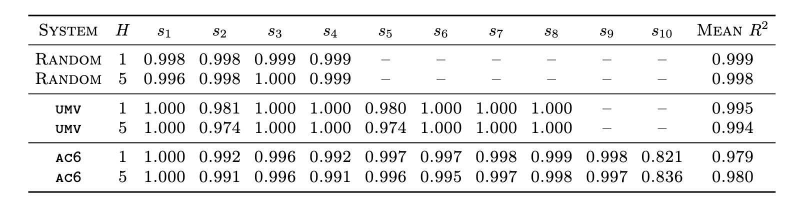
Question: will model activations recover the Kalman filter state estimate, up to similarity transform?
squared loss \( \displaystyle \min \frac{1}{2T} \sum_{t=1}^T \Vert{}y_{t:t+H-1} - G_2 G_1 {z}_t\Vert{}_{2}^2\)
\(z_t:=\)
SS-KF on \(\{u_k, y_k\}_{k=0}^{t-1}\)
Assumptions: Linear-Gaussian system with
similarity transform
model dimension
Proposition (Informal). The optimization landscape is benign.
Yahya Sattar
ICML '26
Theorem (Informal). Let \(d_h=d_x\) and \(H \geq d_x\) and \(L \gtrsim \log(T) / (1 - \rho_\mathrm{KF})\).
filter stability
\(\|S h_t - \hat x_t \|^2 = \|S \hat G_1 z_t - G^\star_1 z_t + G^\star_1 z_t - \hat x_{t|t-1} \|^2\)
$$\hat{x}_{t|t-1} = {G_1^\star} {z}_t + \bar{A}^L \hat{x}_{t-L},\qquad y_{t:t+H-1} ={G_2^\star }\hat{x}_{t|t-1} + \xi_t $$
\(\|S h_t - \hat x_t \|^2 = \|S \hat G_1 z_t - G^\star_1 z_t + G^\star_1 z_t - \hat x_{t|t-1} \|^2\)
properties of optimal KF
truncation error, decays geometrically in \(L\)
Theorem: in-sample prediction error $$\lesssim H\left(d_x (H d_{{y}} + d_{{z}}) + \log \left(\frac{T}{\delta}\right)\right)$$
Theorem: persistent excitation $$\sum_{t=1}^T z_t z_t^\top \succsim T I$$
$$\hat{x}_{t|t-1} = {G_1^\star} {z}_t + \bar{A}^L \hat{x}_{t-L},\qquad y_{t:t+H-1} ={G_2^\star }\hat{x}_{t|t-1} + \xi_t $$
\(\|S h_t - \hat x_t \|^2 = \|S \hat G_1 z_t - G^\star_1 z_t + G^\star_1 z_t - \hat x_{t|t-1} \|^2\)
Theorem (Informal). Let \(d_h=d_x\) and \(H \geq d_x\) and \(L \gtrsim \log(T) / (1 - \rho_\mathrm{KF})\).
$$\min_{S\in\text{GL}_{d_x}(\mathbb R)}\Vert{}Sh_t-\hat{x}_{t|t-1}\Vert{}_{2}^2 \lesssim \epsilon$$
1. Sequences have low rank auto-regressive structure
\(y_{t:t+H-1} \approx G_2^\star G_1^\star {z}_t\)
2. Small prediction errors imply small parameter errors (excitation)
\(\hat G_2\hat G_1 z_t \approx G_2^\star G_1^\star z_t \) for all \(t\)
\(\implies\)
\(\hat G_2\hat G_1 \approx G_2^\star G_1^\star \)
Three ingredients:
\(z_t\)
$$\min \frac{1}{2T} \sum_{t=1}^T \Vert{}y_{t:t+H-1} - G_2 G_1 {z}_t\Vert{}_{2}^2$$
3. Small end-to-end errors imply small first layer errors
\(\hat G_2\hat G_1 \approx G_2^\star G_1^\star \)
\(\implies\)
\(S\hat G_1 \approx G_1^\star \)
filter
controller
\(y\)
\(u\)
system
\(x\)
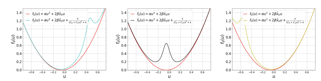
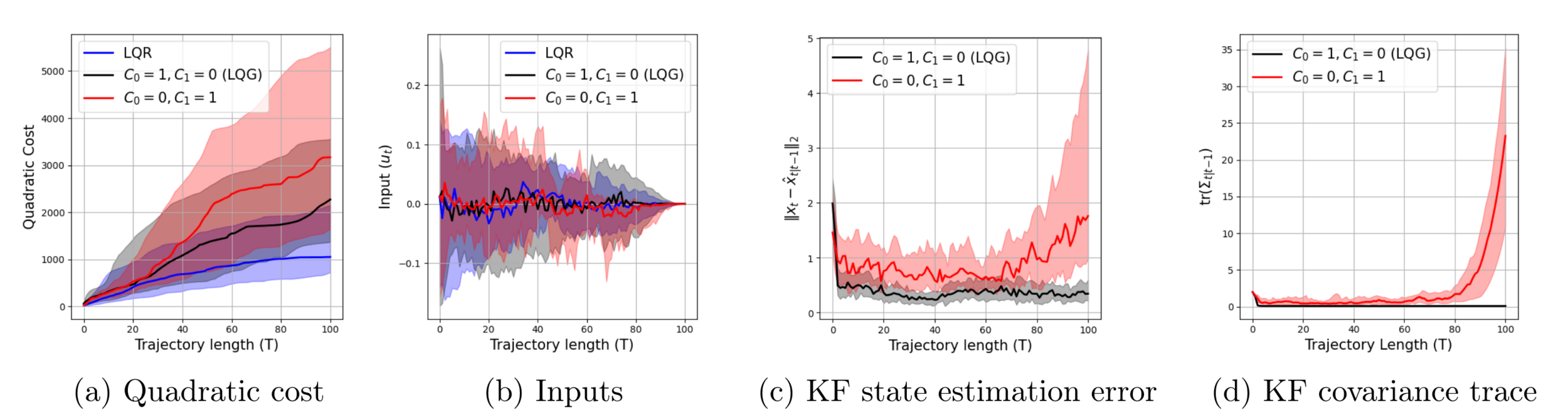
Observer effects occur when there is coupling between actuation and observation
Belief state via the Kalman Filter: \(x_t|\mathcal I_t \sim \mathcal N(\hat x_t,\Sigma_t)\)
\(\hat x_{t+1} = A\hat x_t + Bu_t - L_t\big(y_t-C(u_t)\hat x_t\big)\)
\(\Sigma_{t+1} = (A+ L_tC(u_t))\Sigma_tA^\top + \Sigma_w\)
\(L_t = -A\Sigma_tC(u_t)^\top(C(u_t)\Sigma_tC(u_t)^\top+\Sigma_v)^{-1}\)
$$\min_{u_t=\pi_t(\mathcal I_t)} \mathbb E\left[x_T^\top Q x_T+ \sum_{t=1}^{T-1} x_t^\top Q x_t + u_t^\top R u_t \right]\\ \text{s.t.} \quad x_{t+1} = Ax_t + Bu_t + w_t \\\qquad\qquad\qquad y_t =\Big(C_0 + \sum_{i=1}^p u_t[i] C_i \Big)x_t + v_t$$
Small departure from classic LQG control
Sunmook Choi
Yahya Sattar
Yassir Jedra
Maryam Fazel
Leo Maynard-Zhang
$$\mathcal I_t = \{u_0,...,u_{t-1}, y_0, ..., y_{t-1}\}$$ information set for decision-making
quadratic costs (\(Q,R\succ 0\))
Kalman
Filter
State Feedback
\(y\)
\(\hat x\)
\(u\)
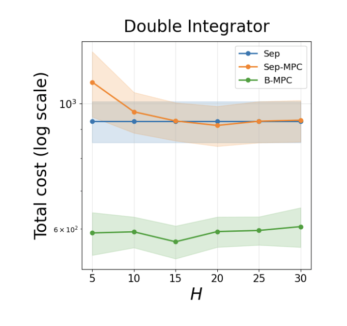
$$\begin{align*} x_{t+1} &= \begin{bmatrix} 1 & 0.3 \\ 0 & 1\end{bmatrix} x_t + \begin{bmatrix}0.3 \\ 0 \end{bmatrix} u_t + w_t \\ y_t &= u_t\begin{bmatrix} 1 & 0\end{bmatrix} x_t + v_t \end{align*}$$
with \(Q=I\) and \(R=1000\)
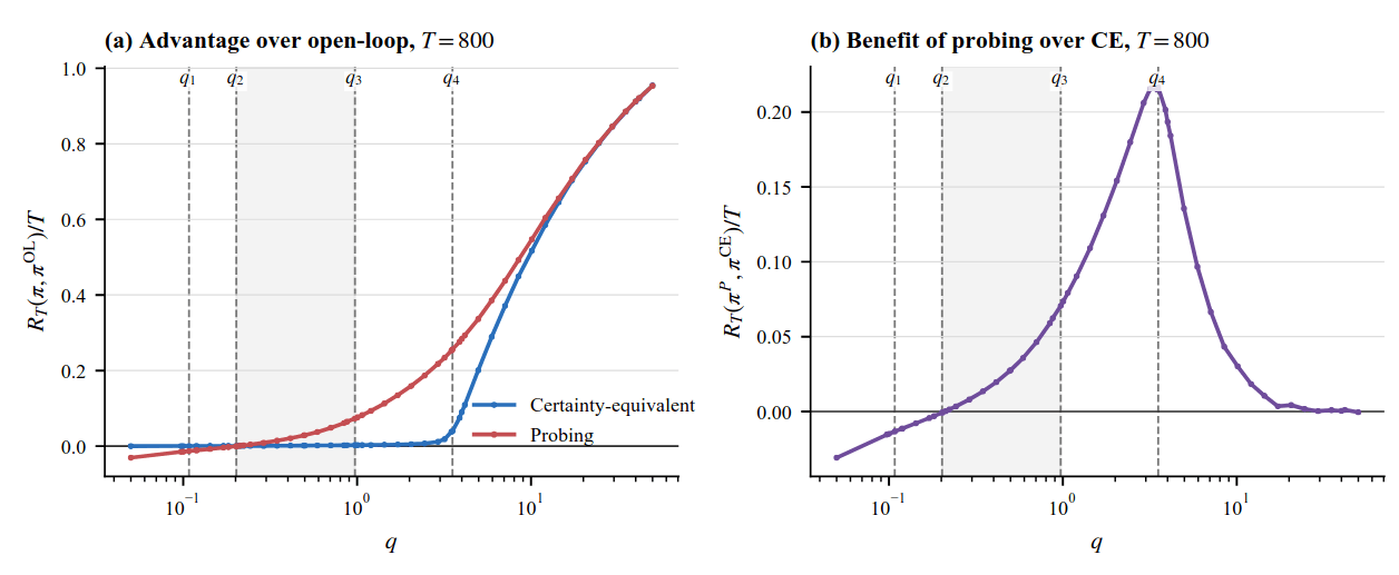
$$\begin{align*} x_{t+1} &= x_t + \begin{bmatrix}0 & 1 \end{bmatrix} u_t + w_t \\ y_t &= u_t^\top \begin{bmatrix} 1\\ 0\end{bmatrix} x_t + v_t \end{align*}$$
with \(Q=\frac{1}{2}\) and \(R=I\)
\(\implies\)
infinite horizon \(K_\star = \begin{bmatrix} 0 \\ \frac{1}{2}\end{bmatrix}\)
\(y_t = \hat x_t \begin{bmatrix} 0 \\ \frac{1}{2}\end{bmatrix}^\top \begin{bmatrix} 1 \\ 0\end{bmatrix} x_t + v_t\)
\(0\) only noise is observed!
\(\propto 1/\sigma_z^2\)
\(\propto 1/\sigma_z^2\)
open loop steady-state covariance
Leo Maynard-Zhang
Sunmook Choi
Yahya Sattar
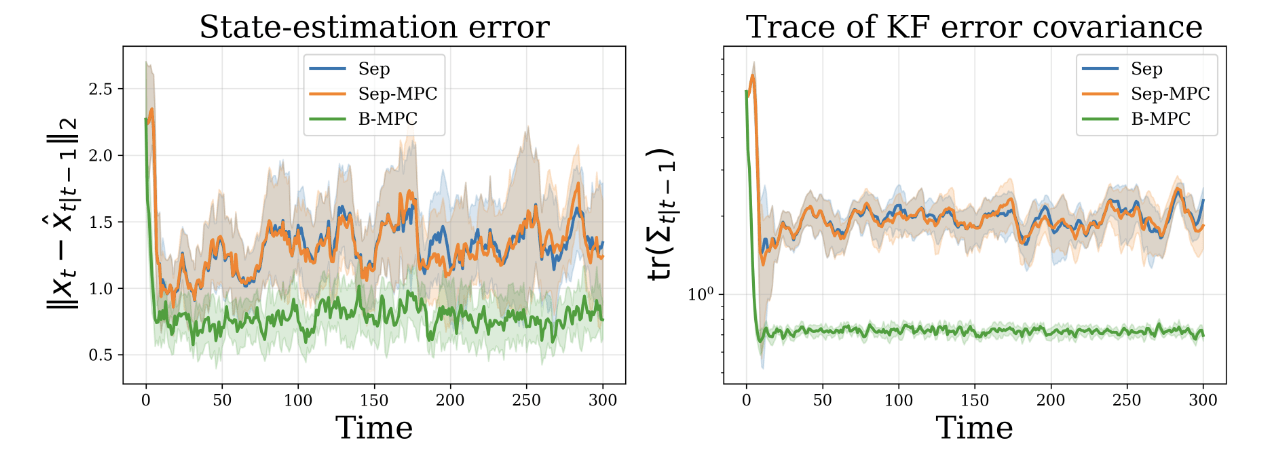
$$\begin{align*}\min_{u_t=\pi_t(\hat x_t,\Sigma_t)}~~& \mathbb E\left[ \sum_{t=1}^{T-1} \hat x_t^\top Q \hat x_t + \mathrm{tr}(\Sigma_t) + u_t^\top R u_t \right]\\ \text{s.t.}~~& \hat x_{t+1} = A\hat x_t + Bu_t + L_t(C(u_t)\hat x_t - y_t)\\ &\Sigma_{t+1} = (A+ L_tC(u_t))\Sigma_tA^\top + \Sigma_w \end{align*}$$
$$\mathbb E\left[x_t^\top Q x_t \mid \mathcal I_t \right]= \hat x_t\top Q\hat x_t + \mathrm{tr}(Q\Sigma_t)$$
$$\begin{align*} \min_{u_t=\pi_t(\mathcal I_t)} ~~&\mathbb E\left[\sum_{t=1}^{T-1} x_t^\top Q x_t + u_t^\top R u_t \right]\\ \text{s.t.}~~& x_{t+1} = Ax_t + Bu_t + w_t \\& y_t =C(u_t)x_t + v_t\end{align*}$$
\(L_t = -A\Sigma_tC(u_t)^\top(C(u_t)\Sigma_tC(u_t)^\top+\Sigma_v)^{-1}\)
Andrew Lowitt
Beixi Du
Daniel Cao
Rewrite OCP in terms of the belief space from KF
This is now a fully observed, nonlinear, stochastic optimal control problem
innovations \(\sim \mathcal N(0, C(u_t)\Sigma_t C(u_t)^\top + \Sigma_v)\)
$$\begin{align*}\pi(\hat x_t,\Sigma_t)=\arg \min_{u_k}~~& \mathbb E\left[ \sum_{k=1}^{H} \bar x_k^\top Q \bar x_k + \mathrm{tr}(\bar\Sigma_k) + u_k^\top R u_k \right]\\ \text{s.t.}~~& \bar x_{k+1} = A\bar x_k + Bu_k\\ &\bar\Sigma_{k+1} = (A+ L_kC(u_k))\Sigma_kA^\top + \Sigma_w \\ &\bar x_0 = \hat x_t ,~~ \bar \Sigma_0=\Sigma_t\end{align*}$$
\(L_t = -A\Sigma_tC(u_t)^\top(C(u_t)\Sigma_tC(u_t)^\top+\Sigma_v)^{-1}\)
Rewrite OCP in terms of the belief space from KF
Expected dynamics, open loop inputs, finite horizon \(\rightarrow\) MPC
"Solve" MPC problem with autograd and L-BFGS
Sunmook Choi
Yahya Sattar
Yassir Jedra
Maryam Fazel
Leo Maynard-Zhang
Andrew Lowitt
Beixi Du
Daniel Cao
Yijia Dai
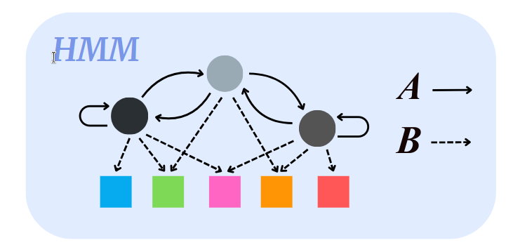
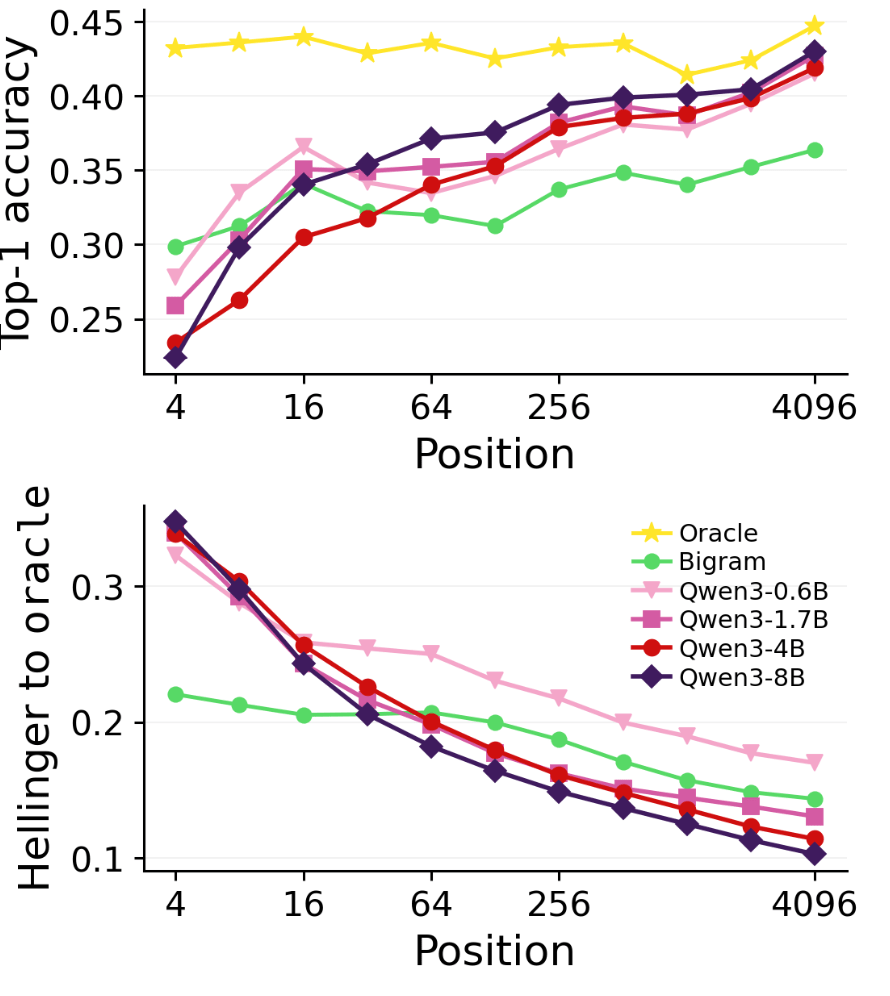
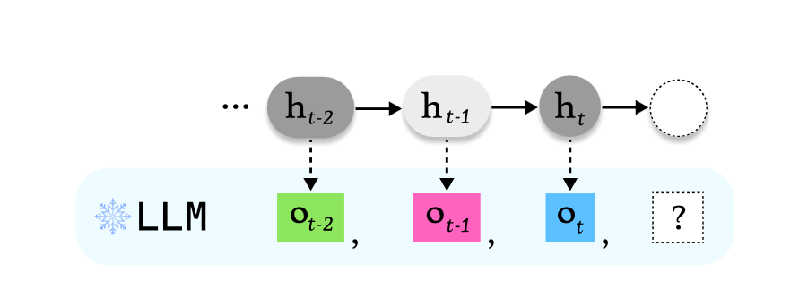
Dai et al., Pre-trained Large Language Models Learn Hidden Markov Models In-context
Sattar et al., Two-Layer Linear Auto-Regressive Models Estimate Latent States
\(x\)
\(A, B\)
\(C\)
\(w\)
\(v\)
\(u\)
\(y\)
Sunmook Choi
Leo Maynard-Zhang
By Sarah Dean