











































Andreas Park PRO
Professor of Finance at UofT
SMU & NTU Seminars 2026
Disclaimer: In the general AMM theory section I am using results from two other papers: "Learning from DeFi" (2024) and "A Simple Theory of Portfolio Market Making (2026), both with Katya Malinova
denarius
sterling
USD
???
Roman Empire
British imperial trade
post-Bretton Woods
"Pax" Americana
1944-
multi-lateral stablecoins
Florin
Medici
MXN
USD
THB
today: routing through the vehicle; two legs, two spreads, two fees
what they want: direct conversion
Trading demand is given; fees cover LPs’ expected losses.
Two things matter: return correlation and cross-pair volume.
We characterize when a cost-minimizing fee schedule can deter such entry.
1
2
3
Not only currencies: any assets traded against cash, e.g. tokenized stocks.
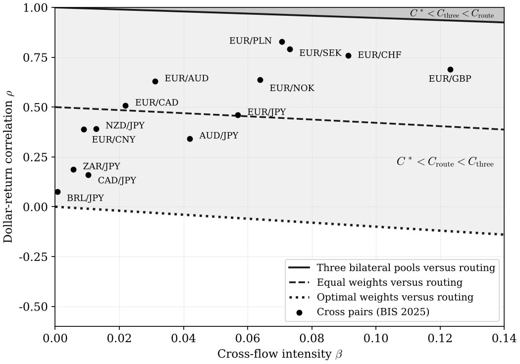
Above the dotted line
Optimal pooling beats dollar routing.
Between dotted and dashed
The capital weights matter.
Higher correlation and more cross-pair flow favor pooling.
92 currencies, many small
13 currencies, all major
| Pair | Cross-trade saving vs USD |
|---|---|
| EUR/SEK | 64% |
| EUR/NOK | 58% |
| EUR/CHF | 57% |
| EUR/GBP | 52% |
| EUR/AUD | 51% |
| NZD/JPY | 46% |
| ZAR/JPY | 45% |
| EUR/CAD | 44% |
| BRL/JPY | 43% |
| EUR/JPY | 40% |
| AUD/JPY | 38% |
| EUR/CNY | 35% |
| CAD/JPY | 30% |
July 31, 2025: "today I am announcing the launch of “Project Crypto”—a Commission-wide initiative to modernize the securities rules and regulations to enable America’s financial markets to move on-chain."
Jul 2025 — GENIUS Act
Aug 2025: Liquid staking guidance
payments
stocks, bonds, and options
swaps, CDS, MBS, CDOs
insurance contracts
What would the most efficient financial infrastructure look like?
payments
stocks, bonds, and options
swaps, CDS, MBS, CDOs
insurance contracts
Broker
Exchange
Internalizer
Wholeseller
Darkpool
Venue
Settlement
Investors
payments network
Stock Exchange
Clearing House
custodian
custodian
beneficial ownership record
seller
buyer
Broker
Broker
1
2
4
3
5
6
7
1
4
6
"laptop on to of a blockchain"
"direct on-chain trading"
"rollup based trading"
Our work and this talk is all V2
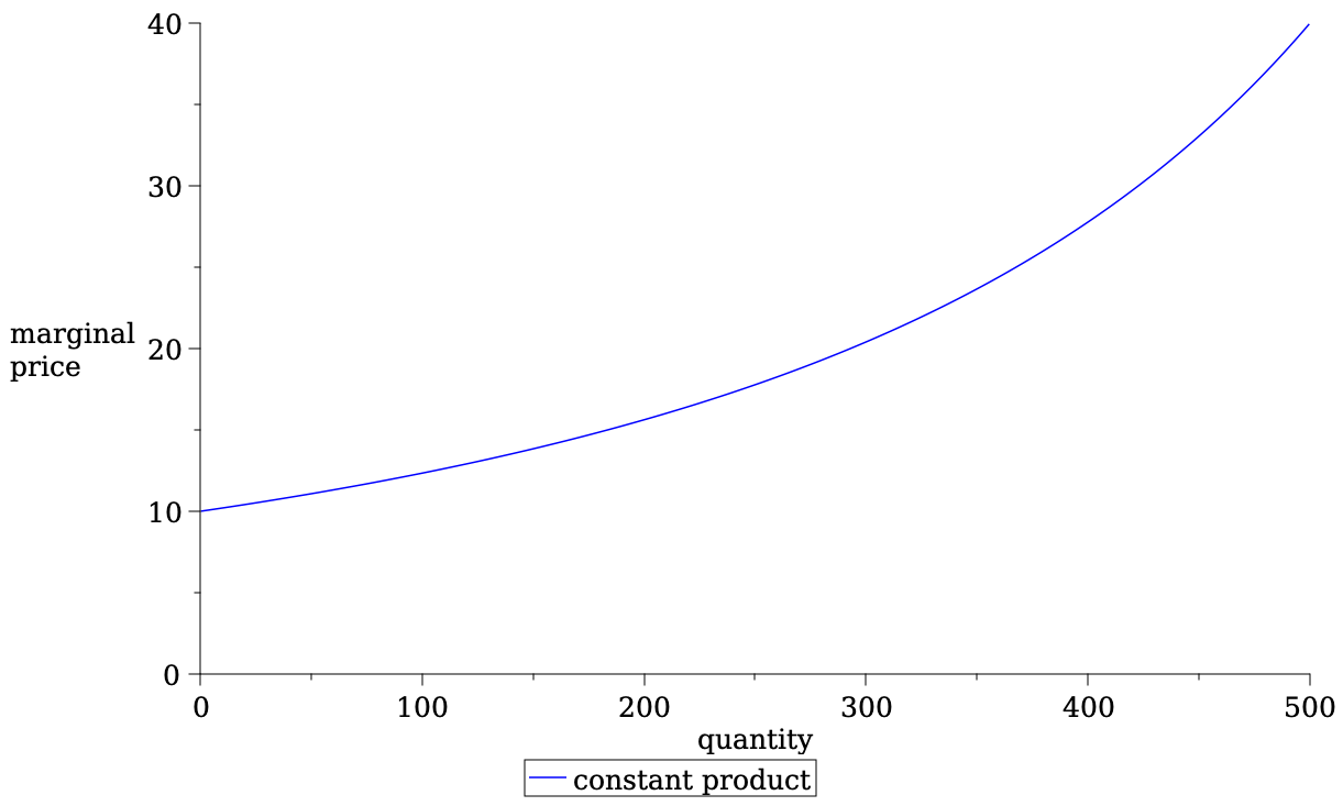
A pool of reserves + a pricing rule \(R_0\cdot R_1=k\). Three things to know:
① Price = slope
S = R₀ / R₁
② Trade walks the curve
price moves → impact
③ LPs shift it out
more depth, same price
A trade ("swap") moves the price along the curve.
Liquidity providers have no positional gains on a round trip → they earn on AMM fees.
Fees accrue on all volume; adverse selection only on the imbalance.
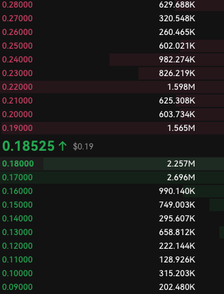
Modern electronic markets are organized as limit order books ...
The math:
... and constant product is a particular limit order book-like price
buy & hold
AMM LP: concave relative to buy & hold
exchange rate change
holding value one currency rel. to other
Proposition: Adverse selection, priced from returns + volume alone.
Our closed form (Learning from DeFi):
\(\mathbb{E}[\text{IL}] = \dfrac{\sigma^2}{8}\)
LPs require compensation for this loss \(\to\) the AMM fee income must cover this loss.
Basic idea of liquidity provision: earn more on balanced flow than what you lose on price movement
\[\text{fee income} +\underbrace{\text{what I sold it for}-\text{value of net position}}_{\text{adverse selection loss}} \ge \text{cost of capital} \]
in AMMs:
protocol fee
in tradFi: bid-ask spread
Pool Designer picks fee \(F\)
A protocol parameter, set at the pool level.
LPs commit liquidity until depth equates \(F\) to expected IL
Competitive break-even provision \(\to\) equilibrium pool size \(D\)
Traders face price impact (liquidity driven) and fee
Deeper pool \(\to\) lower PI for given trade
\[ \min_{F\gt 0} \; F + \frac{\sigma^2 \Delta v}{4F} \]
When period volume is large relative to any single trade:
Optimal fee (per dollar)
\[f^{*}=\frac{\sigma}{2}\sqrt{\frac{\Delta}{v}}\]
Pool depth
\[D^{*}=\frac{4}{\sigma}\sqrt{\Delta v}\]
Cost per dollar traded
\[c^{*}=\sigma\sqrt{\frac{\Delta}{v}}\]
\(\sigma\) = period return volatility — captures adverse selection, reminiscent of the square-root price-impact law
\(v\) = expected "noise" (balanced) volume · \(\Delta\) = representative order size · \(D\) = pool depth
Total fee revenue \(F^*=f^*v=\tfrac{\sigma}{2}\sqrt{\Delta v}\); total cost \(C^*=\sigma\sqrt{\Delta v}\)
For log-return variance \(S=\log(1+\sigma^2)\) over the commitment horizon, total cost for volume \(v\) is
\[\underbrace{C_\ell^*=\sigma\sqrt{\Delta v}}_{\text{local minimum}}\qquad\qquad\underbrace{C_g^*=\sqrt{\Delta v S}}_{\text{global infimum}}\]
Optimized constant product cost
\[ C_{\rm CP,\ell}^*=C_\ell^*,\qquad C_{\rm CP,g}^*=8\sqrt{\frac{\Delta v}{3S}\big(1-e^{-S/8}\big)\big(e^{3S/8}-1\big)}.\]
Excess cost over the commitment horizon
\[ \frac{C_{\rm CP,g}^*}{C_g^*}-1=\frac{\sigma^2}{16}+O(\sigma^4)\qquad (0.0025\%\text{ at }\sigma=2\%;\quad 0.246\%\text{ at }\sigma=20\%).\]
\(\to\) Constant product AMM is "pretty close" to global optimum
An AMM commits to the whole book. Absent news about risk or order flow, its cost benchmarks a discriminatory limit order book à la Glosten (1994).
Kyle (1985), continuous trading
\[\lambda_{\rm Kyle}=\frac{\operatorname{sd}(\text{fundamental return})}{\operatorname{sd}(\text{cumulative noise flow})}=\frac{\sigma}{\sqrt{\Delta v}}\quad\Longrightarrow\quad c^*=\Delta\lambda_{\rm Kyle}.\]
Cost per dollar in the pool
\[c^*=\underbrace{\frac{\sigma^2}{2v\lambda_{\rm Kyle}}}_{\text{fee }f^*:\,\text{LP loss to arbitrage}}+\underbrace{\frac{\Delta\lambda_{\rm Kyle}}{2}}_{\text{average price impact}}=2f^*=\Delta\lambda_{\rm Kyle}.\]
In Kyle, \(\mathbb E[\text{insider profit}]=\lambda_{\rm Kyle}\Delta v=vc^*\), the pool’s total customer cost.
Amihud (2002), empirical illiquidity
\(\displaystyle \mathrm{ILLIQ}=\operatorname{mean}_d\!\left(\frac{|r_d|}{v_d}\right)\): return movement per dollar of volume; for the AMM the denominator is \(\sqrt{\Delta v}\).
Same total capital \(D\): split it across three pools, or pool it.
pool the capital →
each reserve backs both of its pairs
Pool rule: \(a_0^{w_0}\cdot a_1^{w_1}\cdot a_2^{w_2}=\) constant. Weights \(w_i\) = shares of the pool’s value.
each pool: 50–50 weights, capital ⅓ \(D\)
price impact \(\;\dfrac{2\Delta}{\tfrac13 D}=\dfrac{6\Delta}{D}\)
\(\Delta\) = trade size
weights ⅓ each, capital \(D\)
price impact \(\;\dfrac{3\Delta}{D}\)
Illustration: common news raises the values of A and B together. Their quotes are stale until someone trades on the news.
Two separate markets
Arbitrageur
sees the news first
buys A
Pool A
quote stale: gain
buys B
Pool B
also stale: gain
Separate stale-price losses
One portfolio pool
Arbitrageur
sees the news first
buys A
Pool A + B
raises the quote of A, and of B, which moves with it
B also adjusts: less remaining arbitrage
Smaller combined loss
Less adverse selection, less compensation, lower cost. Competitive providers enter until fees cover their expected losses, so what helps them is passed on to investors as lower fees. The pool needs no coordination: the joint update is governed by market infrastructure and part of the trade itself.
As with one risky asset:
With several risky assets:
\[\prod_i a_i^{w_i}=\text{constant}\qquad\sum_i w_i=1 \qquad w_i\gt 0\qquad p_{ij}^{\mathrm{pool}}=\frac{w_i a_j}{w_j a_i}\]
37 ·
total depth is price times deposits but
relative prices also imply \(p_i a_i=Dw_i\)
\[\text{Price impact}_{ij}=\underbrace{\frac12\left(\frac1{w_i}+\frac1{w_j}\right)}_{\text{price impact coefficient}}\frac{\Delta}{D}\]
\[\frac{\Delta\Gamma}{D}\]
\[\begin{aligned}\text{Two assets:}\quad&\mathbb E[\text{LP loss}]\simeq\tfrac12\,w_0w_1\,\sigma^{2}\,D\\[10pt]\text{Many assets:}\quad&\mathbb E[\text{LP loss}]\simeq\tfrac12\,\Phi(w)\,D,\qquad \Phi(w)=\sum_{i<j}w_iw_j\,\sigma_{ij}^{2}\end{aligned}\]
\(\sigma_{ij}\) = volatility of the \(i\)–\(j\) exchange rate. The sum includes dollar pairs.
\[F=\frac12\Phi D\quad\Longrightarrow\quad D=\frac{2F}{\Phi}\]
LPs break even: fees collected \(F\) = LP losses \(\tfrac12\Phi D\) → depth \(D=2F/\Phi\).
Traders pay fees plus price impact:
\[C(F)=\underbrace{F}_{\text{fees}}+\underbrace{\frac{\Gamma\,\Delta}{D}}_{\text{price impact}}=F+\frac{\Delta\,\Phi\,\Gamma}{2F}\]
\(\displaystyle\Gamma(w)=\sum_{i<j}V_{ij}\Big(\frac{1}{2w_i}+\frac{1}{2w_j}\Big)\)
\(f_{ij}\) = fee rate, \(V_{ij}\) = volume traded on pair \(i,j\)
Result: fee schedules that collect the same total give the same depth and the same total trading cost. Two assets: one fee. Many assets: many schedules.
\[C(F;w)=F+\frac{\Delta\Gamma(w)\Phi(w)}{2F}\]
\(\Leftrightarrow\)
\[\begin{aligned}F^*(w)&=\sqrt{\frac{\Delta\Phi(w)\Gamma(w)}2}\\[0.5em]D^*(w)&=\sqrt{\frac{2\Delta\Gamma(w)}{\Phi(w)}}\\[0.5em]C^*(w)&=\sqrt{2\Delta\Phi(w)\Gamma(w)}=2F^*(w)\end{aligned}\]
Proposition 3: For given weights, optimizing Fees and Minimal Costs are
\[C^*=\min_w C^*(w) =\min_{w}\sqrt{2\Delta\Phi\Gamma}\]
\[C^*=\min_w\sum_i\sqrt{\Delta V_i}\,\sigma_{iw}\]
Theorem: The minimized volume-weighted sum of these relative volatilities is
with optimal weights are \(a_i^*=\frac{\sqrt{\Delta V_i}}{p_i\sigma_{i w^*}}\)
Theorem: a multi-asset pool can be designed to achieve lower total trading costs than dollar routing if and only if \(T \gt 0\).
\[T=\underbrace{\sum_{i\lt j}\sqrt{V_iV_j}\,\rho_{ij}}_{\text{how currencies move together}}\;+\;\underbrace{\sum_{i\lt j}v_{ij}}_{\text{cross-pair volume}}\]
\(V_i\) = total volume that currency \(i\)'s dollar market serves under routing
\(\rho_{ij}\) = correlation of dollar returns · \(v_{ij}\) = direct cross-pair demand
Sums over non-dollar currencies.
With two non-dollar currencies, the theorem’s \(T\) becomes:
\[T=\sqrt{V_1V_2}\,(\rho+\beta),\qquad \beta=\frac{v_{12}}{\sqrt{V_1V_2}}\]
\(\rho\): correlation of dollar returns
\(\beta\): cross-pair flow intensity; with equal volumes, the cross-pair share of demand
A pool can be designed to beat routing if and only if \(\rho\gt-\beta\).
More cross-pair demand increases the savings from direct trading. These savings can outweigh the extra LP compensation that negative correlation requires.
Positive correlation lowers the loss from realigning cross rates.
Direct cross-pair trading avoids impact on an intermediate dollar deposit in separate dollar markets.
More cross-flow therefore permits some negative correlation.
above dashed: equal thirds (BIS Project Mariana’s design) beats routing.
above dotted: the optimally weighted pool beats routing: \(\rho > -\beta\).
With no cross-pair flow (\(\beta = 0\)): equal thirds needs \(\rho > 0.5\); optimal weights need only \(\rho > 0\).
above solid: three separate pools beat vehicle routing (but not multi-asset pool)
| Cross-trade cost (bps) | Pool saving vs USD | ||||
|---|---|---|---|---|---|
| Pair | Direct | Via USD | Pool | Cross | Aggregate |
| EUR/SEK | 0.46 | 0.45 | 0.16 | 64% | 9.5% |
| EUR/NOK | 0.80 | 0.60 | 0.25 | 58% | 5.9% |
| EUR/CHF | 0.22 | 0.21 | 0.09 | 57% | 10.0% |
| EUR/GBP | 0.22 | 0.20 | 0.10 | 52% | 9.5% |
| EUR/AUD | 0.64 | 0.27 | 0.13 | 51% | 6.1% |
| NZD/JPY | 2.04 | 0.51 | 0.27 | 46% | 1.6% |
| ZAR/JPY | 5.06 | 0.84 | 0.46 | 45% | 0.4% |
| EUR/CAD | 0.64 | 0.20 | 0.11 | 44% | 3.3% |
| BRL/JPY | 16.52 | 0.86 | 0.49 | 43% | 0.1% |
| EUR/JPY | 0.38 | 0.17 | 0.10 | 40% | 3.5% |
| AUD/JPY | 0.83 | 0.31 | 0.19 | 38% | 1.8% |
| EUR/CNY | 0.89 | 0.14 | 0.09 | 35% | 1.7% |
| CAD/JPY | 1.57 | 0.24 | 0.17 | 30% | 0.3% |
Insight 1: vehicle routing through dollar is cheaper than a direct pool
Insight 2: via the pool, the cross trade is cheaper
Insight 3: the pool on the whole is also cheaper than routing
3,164 pairs, 92 currencies
About 70% pass
30% fail ρ > −β.
Failures: near-zero intensity, slightly negative correlation.
Pass = some cheaper design exists. Not measured savings.
\(\beta=q_{12}/\sqrt{Q_1Q_2}\). The test also holds for unequal volumes and volatilities. Data: Refinitiv 2019–24; IMF DOTS 2019–23 (goods trade).
Theorem: Suppose the optimum is interior and volume positive. There exists a nonnegative fee schedule that raises the required revenue, is internally consistent and prevents every dedicated dollar-pair entrant from offering a strictly lower cost if and only if
*consistency= cross-pair fees cannot exceed the sum of the two within-pool dollar fees.
| Best defensible split | No dollar trader above routing | ||||
|---|---|---|---|---|---|
| Pair | Via USD | Cost | Saving | Cost | Saving |
| EUR/SEK | 0.45 | 0.12 | 74% | 0.12 | 74% |
| EUR/NOK | 0.60 | 0.21 | 65% | 0.21 | 65% |
| EUR/CHF | 0.21 | 0.05 | 75% | 0.05 | 75% |
| EUR/GBP | 0.20 | 0.06 | 73% | 0.06 | 73% |
| EUR/AUD | 0.27 | 0.09 | 68% | 0.09 | 68% |
| NZD/JPY | 0.51 | 0.21 | 59% | 0.21 | 59% |
| ZAR/JPY | 0.84 | 0.39 | 53% | 0.42 | 50% |
| EUR/CAD | 0.20 | 0.07 | 64% | 0.07 | 64% |
| BRL/JPY | 0.86 | 0.42 | 51% | 0.42 | 51% |
| EUR/JPY | 0.17 | 0.06 | 64% | 0.07 | 61% |
| AUD/JPY | 0.31 | 0.12 | 60% | 0.18 | 42% |
| EUR/CNY | 0.14 | 0.05 | 60% | 0.05 | 60% |
| CAD/JPY | 0.24 | 0.11 | 54% | 0.16 | 32% |
One-way cost in bps of a $5M cross trade; savings relative to routing via USD.
Cost of vehicle routing
the best scenario for the cross pool relative to routing that is defensible
the best defensible scenario for the cross pool where no pair costs more than under routing
\[\begin{aligned}\Phi&=\sum_{i<j}w_iw_j\sigma_{ij}^2\\[0.4em]\Gamma&=\frac12\sum_i\frac{V_i}{w_i}\end{aligned}\]
\(\sigma_{ij}^2=\operatorname{Var}(\varepsilon_i-\varepsilon_j)\) includes dollar pairs.
Expected loss is \(\frac12\Phi D\). Aggregate price impact is \(\Delta\Gamma/D\).
For fixed reference \(\alpha\), each deposit minimizes its own impact-plus-risk term.
Conditional dollar deposit: \(p_i a_i=\sqrt{\Delta V_i}/\sigma_{i\alpha}\).
The auxiliary objective equals actual cost plus a nonnegative mismatch term.
\[\text{Mismatch}=\frac12D\operatorname{Var}\!\left[(w-\alpha)^\prime\varepsilon\right]\]
Start at the dollar reference. For small \(t>0\), set \(\alpha_i(t)=t\sqrt{V_i}/\sigma_i\).
Set \(\alpha_0(t)\) so that weights sum to one.
After omitting the positive factor \(\sqrt{\Delta}\), the derivative is:
\[\sqrt{V_0+2T}\left[\sqrt{V_0}-\sqrt{V_0+2T}\right]\]
It is negative if and only if \(T>0\).
\[w_0^*=\sqrt{\frac{(1-\rho)(1-\beta)}{(1+\rho)(1+\beta)}}\]
\(V_1=V_2=V\) and \(\sigma_1=\sigma_2=\sigma\).
\(v_{12}=\beta V\), so cross-flow share equals cross-flow intensity.
\(w_1^*=w_2^*=(1-w_0^*)/2\).
\(\omega_i\) = entrant cost − incumbent dollar-pair impact.
Need \(\omega_i\ge0\) for every \(i\), and \(\sum_i V_i\omega_i\ge F^*\).
Choose dollar fees in proportion to \(\omega_i\) to raise \(F^*\).
Set each cross fee to the sum of its two dollar fees.
Underlying pair demands and average trade size.
The currencies assigned to the pool and the geometric-mean rule.
Competitive liquidity supply and an external efficient-price process.
Extensions include elastic demand, pool membership and competition among trading routes.
MXN
USD
THB
MXN
USD
THB
USD
MXN
THB
Status Quo (SQ)
Two bilateral USD pools. MXN/THB route through USD
Three Bilateral Pools (BP)
One pool per pair. No forced routing but fragmented capital and volume
Single multilateral pool (MP)
all three currencies in one pool; direct trading of all pairs
Same approach as single pool: LP break even, cost-minimizing planner
Split the capital and each pair gets a book only ⅓ as deep — price impact rises. Pool it, and every dollar backs all three pairs.
⅓ D
⅓ D
⅓ D
USD/MXN
USD/THB
MXN/THB
capital split 3 ways
pool the capital →
D
every dollar backs all 3 pairs
price impact, split capital:
\[\frac{2\Delta}{D/3}=\frac{6\Delta}{D}\]
price impact, pooled:
\[\frac{2\Delta}{\frac{2}{3}D}=\frac{3\Delta}{D}\]
liquidity invariant (equal weights) \[R_0\cdot R_1\cdots R_n = k\]
marginal rate vs numeraire \((S_0\equiv 1)\) \[S_i=\frac{R_0}{R_i}\]
pool depth (at market prices) \[D=\sum_i S_i R_i = n\,R_0\]
Lemma (equal thirds). Each currency holds one third of pool depth: \(\;S_i R_i = \dfrac{D}{3}\)
Price impact. A trade \(i\to j\) touches 2 of 3 currencies — backed by \(\tfrac{2}{3}D\):
\[\Pi=\frac{2\Delta}{\frac{2}{3}D}=\frac{3\Delta}{D}\]
Impermanent loss— our closed-form approximation:
\[\mathbb{E}[\text{IL}]=\frac{\Sigma}{18},\quad \Sigma=\sigma_{01}^2+\sigma_{02}^2+\sigma_{12}^2\]
extends bilateral \(\;\sigma^2/8\) · this is what the AMM fee must cover
① LPs commit liquidity
until fee revenue covers expected IL — this pins down depth D.
② Designer picks fee F
to minimize price impact + fee — depth substitutes out, leaving the cost.
A trade ("swap") moves the price along the curve.
Liquidity providers have no positional gains on a round trip → they earn on AMM fees.
Fees accrue on all volume; adverse selection only on the imbalance.
buy & hold
AMM LP: concave relative to buy & hold
exchange rate change
holding value one currency rel. to other
Proposition: Adverse selection, priced from returns + volume alone.
Our closed form (Learning from DeFi):
\(\mathbb{E}[\text{IL}] = \dfrac{\sigma^2}{8}\)
The AMM fee must cover it.
Competitive, risk-neutral liquidity providers can enter and exit freely.
Traders have fixed pair demands and a common small trade size \(\Delta\).
Arbitrage aligns terminal pool quotes with external exchange rates.
Small trades and small returns give tractable cost approximations.
By Andreas Park
My slides for seminars at SMU and NTU in Singapore in November 2026.