59th NATIONAL CONGRESS OF THE MEXICAN MATHEMATICAL SOCIETY · NUMERICAL METHODS SESSION
Numerical simulation and maximum likelihood estimation for a
stochastic advection-diffusion equation
Saúl Díaz-Infante (SECIHTI – Universidad de Sonora) · saul.diazinfante@unison.mx
Joint work with Fernando Baltazar-Larios (UNAM), Francisco Delgado-Vences (UAB, Barcelona)
and Gerardo Hernández-Dueñas (IM-UNAM, Juriquilla)
Tlaxcala, October 2026
Motivation: transport under uncertainty
Advection-diffusion: transport of a passive tracer (pollutant, heat, biomass) by a flow plus diffusion.
Real systems are noisy: turbulence, unresolved scales, environmental forcing → SPDE.
Inverse problem: from observed dynamics, estimate the diffusion \(\beta\) and the advection coupling \(\theta\).
What is new?
Classical spectral MLE assumes diagonal systems: each Fourier mode is an independent OU process.
A velocity field couples all modes: we must estimate from an infinite system of coupled SDEs.
\begin{cases} {\color{#162D54}du}\mathrel{\color{#162D54}=}{\color{#162D54}\big[}{\color{#162D54}\beta}{\color{#0077B6}\,\boldsymbol{\Delta} u}\mathbin{\color{#162D54}-}{\color{#162D54}\theta}{\color{#0077B6}\,\bar{\mathbf v}}{\color{#0077B6}\cdot\nabla u}{\color{#162D54}\big]\,dt}\mathbin{\color{transparent}+}{\color{transparent}\sigma}{\color{transparent}\displaystyle\sum_{k\in\mathbb N}\lambda_k^{-\gamma}\,h_k(x)\,dw_k(t)}{\color{#162D54},} & {\color{#162D54}\text{in } (0,T]\times\mathcal O,}\\[6pt] {\color{#162D54}\dfrac{\partial u}{\partial\eta}=0,} & {\color{#162D54}\text{on } [0,T]\times\partial\mathcal O,}\\[6pt] {\color{#162D54}u(0,x)=u_0(x),} & {\color{#162D54}\text{in } \mathcal O.} \end{cases}
\begin{cases} {\color{transparent}du}\mathrel{\color{transparent}=}{\color{transparent}\big[}{\color{transparent}\beta}{\color{transparent}\,\boldsymbol{\Delta} u}\mathbin{\color{transparent}-}{\color{transparent}\theta}{\color{transparent}\,\bar{\mathbf v}}{\color{transparent}\cdot\nabla u}{\color{transparent}\big]\,dt}\mathbin{\color{#2A9D5C}+}{\color{#2A9D5C}\sigma}{\color{#2A9D5C}\displaystyle\sum_{k\in\mathbb N}\lambda_k^{-\gamma}\,h_k(x)\,dw_k(t)}{\color{transparent},} & {\color{transparent}\text{in } (0,T]\times\mathcal O,}\\[6pt] {\color{transparent}\dfrac{\partial u}{\partial\eta}=0,} & {\color{transparent}\text{on } [0,T]\times\partial\mathcal O,}\\[6pt] {\color{transparent}u(0,x)=u_0(x),} & {\color{transparent}\text{in } \mathcal O.} \end{cases}
\begin{cases} {\color{transparent}du}\mathrel{\color{transparent}=}{\color{transparent}\big[}{\color{#E07A1F}\beta}{\color{transparent}\,\boldsymbol{\Delta} u}\mathbin{\color{transparent}-}{\color{#E07A1F}\theta}{\color{transparent}\,\bar{\mathbf v}}{\color{transparent}\cdot\nabla u}{\color{transparent}\big]\,dt}\mathbin{\color{transparent}+}{\color{transparent}\sigma}{\color{transparent}\displaystyle\sum_{k\in\mathbb N}\lambda_k^{-\gamma}\,h_k(x)\,dw_k(t)}{\color{transparent},} & {\color{transparent}\text{in } (0,T]\times\mathcal O,}\\[6pt] {\color{transparent}\dfrac{\partial u}{\partial\eta}=0,} & {\color{transparent}\text{on } (0,T]\times\partial\mathcal O,}\\[6pt] {\color{transparent}u(0,x)=u_0(x),} & {\color{transparent}\text{in } \mathcal O.} \end{cases}
The model
\begin{cases} {\color{#162D54}du}\mathrel{\color{#162D54}=}{\color{#162D54}\big[}{\color{#E07A1F}\beta}{\color{#0077B6}\,\boldsymbol{\Delta}}{\color{#0077B6}u}\mathbin{\color{#162D54}-}{\color{#E07A1F}\theta}{\color{#0077B6}\,\bar{\mathbf v}}{\color{#0077B6}\cdot\nabla u}{\color{#162D54}\big]\,dt}\mathbin{\color{#2A9D5C}+}{\color{#2A9D5C}\sigma}{\color{#2A9D5C}\displaystyle\sum_{k\in\mathbb N}}{\color{#2A9D5C}\lambda_k^{-\gamma}}{\color{#2A9D5C}\,h_k(x)}{\color{#2A9D5C}\,dw_k(t)}{\color{#162D54},} & {\color{#162D54}\text{in } (0,T]\times\mathcal O,}\\[6pt] {\color{#162D54}\dfrac{\partial u}{\partial\eta}=0,} & {\color{#162D54}\text{on } [0,T]\times\partial\mathcal O,}\\[6pt] {\color{#162D54}u(0,x)=u_0(x),} & {\color{#162D54}\text{in } \mathcal O.} \end{cases}
\begin{cases} {\color{transparent}du}\mathrel{\color{transparent}=}{\color{transparent}\big[}{\color{transparent}\beta}{\color{transparent}\,\boldsymbol{\Delta}}{\color{transparent}u}\mathbin{\color{transparent}-}{\color{transparent}\theta}{\color{transparent}\,\bar{\mathbf v}}{\color{transparent}\cdot\nabla u}{\color{transparent}\big]\,dt}\mathbin{\color{transparent}+}{\color{transparent}\sigma}{\color{transparent}\displaystyle\sum_{k\in\mathbb N}}{\color{transparent}\lambda_k^{-\gamma}}{\color{transparent}\,h_k(x)}{\color{transparent}\,dw_k(t)}{\color{transparent},} & {\color{transparent}\text{in } (0,T]\times\mathcal O,}\\[6pt] {\color{#D62828}\dfrac{\partial u}{\partial\eta}=0,} & {\color{#D62828}\text{on } [0,T]\times\partial\mathcal O,}\\[6pt] {\color{#D62828}u(0,x)=u_0(x),} & {\color{transparent}\text{in } \mathcal O.} \end{cases}
\begin{cases} {\color{transparent}du}\mathrel{\color{transparent}=}{\color{transparent}\big[}{\color{transparent}\beta}{\color{transparent}\,\boldsymbol{\Delta}}{\color{transparent}u}\mathbin{\color{transparent}-}{\color{transparent}\theta}{\color{#D62828}\,\bar{\mathbf v}}{\color{transparent}\cdot\nabla u}{\color{transparent}\big]\,dt}\mathbin{\color{transparent}+}{\color{transparent}\sigma}{\color{transparent}\displaystyle\sum_{k\in\mathbb N}}{\color{transparent}\lambda_k^{-\gamma}}{\color{transparent}\,h_k(x)}{\color{transparent}\,dw_k(t)}{\color{transparent},} & {\color{transparent}\text{in } (0,T]\times\mathcal O,}\\[6pt] {\color{transparent}\dfrac{\partial u}{\partial\eta}=0,} & {\color{transparent}\text{on } [0,T]\times\partial\mathcal O,}\\[6pt] {\color{transparent}u(0,x)=u_0(x),} & {\color{transparent}\text{in } \mathcal O.} \end{cases}
\begin{cases} {\color{transparent}du}\mathrel{\color{transparent}=}{\color{transparent}\big[}{\color{transparent}\beta}{\color{#D62828}\,\boldsymbol{\Delta}}{\color{transparent}u}\mathbin{\color{transparent}-}{\color{transparent}\theta}{\color{transparent}\,\bar{\mathbf v}}{\color{transparent}\cdot\nabla u}{\color{transparent}\big]\,dt}\mathbin{\color{transparent}+}{\color{transparent}\sigma}{\color{transparent}\displaystyle\sum_{k\in\mathbb N}}{\color{#D62828}\lambda_k^{-\gamma}}{\color{#D62828}\,h_k(x)}{\color{#D62828}\,dw_k(t)}{\color{transparent},} & {\color{transparent}\text{in } (0,T]\times\mathcal O,}\\[6pt] {\color{transparent}\dfrac{\partial u}{\partial\eta}=0,} & {\color{transparent}\text{on } [0,T]\times\partial\mathcal O,}\\[6pt] {\color{transparent}u(0,x)=u_0(x),} & {\color{transparent}\text{in } \mathcal O.} \end{cases}
\begin{cases} {\color{transparent}du}\mathrel{\color{transparent}=}{\color{transparent}\big[}{\color{transparent}\beta}{\color{transparent}\,\boldsymbol{\Delta}}{\color{transparent}u}\mathbin{\color{transparent}-}{\color{transparent}\theta}{\color{transparent}\,\bar{\mathbf v}}{\color{transparent}\cdot\nabla u}{\color{transparent}\big]\,dt}\mathbin{\color{transparent}+}{\color{transparent}\sigma}{\color{transparent}\displaystyle\sum_{k\in\mathbb N}}{\color{#D62828}\lambda_k^{-\gamma}}{\color{transparent}\,h_k(x)}{\color{transparent}\,dw_k(t)}{\color{transparent},} & {\color{transparent}\text{in } (0,T]\times\mathcal O,}\\[6pt] {\color{transparent}\dfrac{\partial u}{\partial\eta}=0,} & {\color{transparent}\text{on } [0,T]\times\partial\mathcal O,}\\[6pt] {\color{transparent}u(0,x)=u_0(x),} & {\color{transparent}\text{in } \mathcal O.} \end{cases}
Homogeneous Neumann (zero-flux) condition; \(u_0\in\mathcal H\).
Steady, incompressible velocity: \(\nabla\cdot\bar{\mathbf v}=0\), no penetration \(\bar{\mathbf v}\cdot\mathbf n=0\) on \(\partial\mathcal O\).
\((\lambda_k,h_k)\): Neumann eigenpairs of \(-\boldsymbol{\Delta}\) (next slide); \(\{w_k\}_{k\ge1}\) independent standard Wiener processes.
Noise white in time, colored in space: \(\lambda_k^{-\gamma}\) damps high modes (trace class).
| Parameter | Role |
| \({\color{#E07A1F}\beta}>0\) | diffusion |
| \({\color{#E07A1F}\theta}\in[0,1]\) | advection coupling |
| \({\color{#2A9D5C}\sigma}\ge 0\) | noise intensity |
| \(\gamma\in[0,1]\) | spatial regularity of noise |
Linear in \(u\); \(\theta\) absorbs uncertainty in the measured flow.
Additive noise may produce negative concentrations: a deliberate baseline to isolate the effect of modal coupling.
Spectral setting: eigen-expansion of the Laplacian
\begin{cases} -\boldsymbol{\Delta} h_k=\lambda_k\,h_k, & \text{in } \mathcal O,\\[6pt] \dfrac{\partial h_k}{\partial\eta}=0, & \text{on } \partial\mathcal O, \end{cases}\qquad k\in\mathbb N\cup\{0\}
Grebenkov, D. S., & Nguyen, B.-T. (2013). Geometrical structure of Laplacian eigenfunctions. SIAM Review, 55(4), 601–667. https://doi.org/10.1137/120880173
Ivrii, V. (2016). 100 years of Weyl's law. Bulletin of Mathematical Sciences, 6(3), 379–452. https://doi.org/10.1007/s13373-016-0089-y
Reed, M., & Simon, B. (1978). Methods of Modern Mathematical Physics IV: Analysis of Operators (Sect. XIII.15). Academic Press. ISBN 978-0-12-585004-9
(i) \(\{h_k\}_{k\in\mathbb N\cup\{0\}}\) is an orthonormal basis of \(L^2(\mathcal O)\).
(ii) Discrete spectrum (Reed & Simon, 1978):
\[0=\lambda_0<\lambda_1\le\lambda_2\le\cdots\to+\infty .\]
(iii) \(h_0\) is constant (mass conservation); we work in
\[\mathcal H=h_0^{\perp}\subset L^2(\mathcal O).\]
(iv) Weyl's law (Ivrii, 2016; Grebenkov & Nguyen, 2013, §4.1):
\[\lim_{k\to\infty}\lambda_k\,k^{-2/d}=\varpi>0 .\]
Spectral expansion, \(u_k=(u,h_k)_{\mathcal H}\):
\[u=\sum_{k}u_k h_k,\qquad -\boldsymbol{\Delta} u=\sum_{k}\lambda_k u_k h_k,\]
hence diagonal action:
\[Bh_k=\lambda_k^{-\gamma}h_k,\quad S(t)h_k=e^{t\beta\boldsymbol{\Delta}}h_k=e^{-\beta\lambda_k t}h_k .\]
Basis in the paper, \(\mathcal O=[0,L_1]\times[0,L_2]\):
\[h_{(i,j)}=\sqrt{2-\delta_{i,0}}\sqrt{2-\delta_{j,0}}\,\cos\tfrac{\pi i x}{L_1}\cos\tfrac{\pi j y}{L_2},\]
\[\lambda_{(i,j)}=\pi^2\Big(\frac{i^2}{L_1^2}+\frac{j^2}{L_2^2}\Big),\quad i,j\in\mathbb N\cup\{0\} .\]
Multi-index label (\(i\) acts on \(x\), \(j\) on \(y\)), ordered by eigenvalue:
\[k=k(i,j),\qquad h_k=h_{(i,j)},\qquad \lambda_k=\lambda_{(i,j)} .\]
Cylindrical Brownian motion (Da Prato & Zabczyk, 1992)
Definition. Let \(\{w_k\}_{k\ge1}\) be independent standard Wiener processes and \(\{h_k\}_{k\ge1}\) the orthonormal basis of \(\mathcal H\). The cylindrical Brownian motion on \(\mathcal H\) is the formal series
W(t)=\sum_{k=1}^{\infty} w_k(t)\, h_k, \qquad t\ge 0
Da Prato, G., & Zabczyk, J. (1992). Stochastic Equations in Infinite Dimensions (Encyclopedia of Mathematics and its Applications, Vol. 44). Cambridge University Press. https://doi.org/10.1017/CBO9780511666223
(i) A \(Q\)-Wiener process with \(Q=I\), not convergent in \(\mathcal H\):
\[\mathbb E\,\|W(t)\|_{\mathcal H}^2=\sum_{k\ge1} t=\infty .\]
(ii) Its coordinates are real Wiener processes:
\[\mathbb E\big[(W(t),f)_{\mathcal H}(W(s),g)_{\mathcal H}\big]=(t\wedge s)\,(f,g)_{\mathcal H}.\]
(iii) In our model, with \(Bh_k=\lambda_k^{-\gamma}h_k\):
\[\sigma\sum_{k\in\mathbb N}\lambda_k^{-\gamma}h_k\,dw_k(t)=\sigma B\,dW(t),\]
\[\operatorname{Tr}(BB^{*})=\sum_{k}\lambda_k^{-2\gamma}<\infty\iff\gamma>d/4 .\]
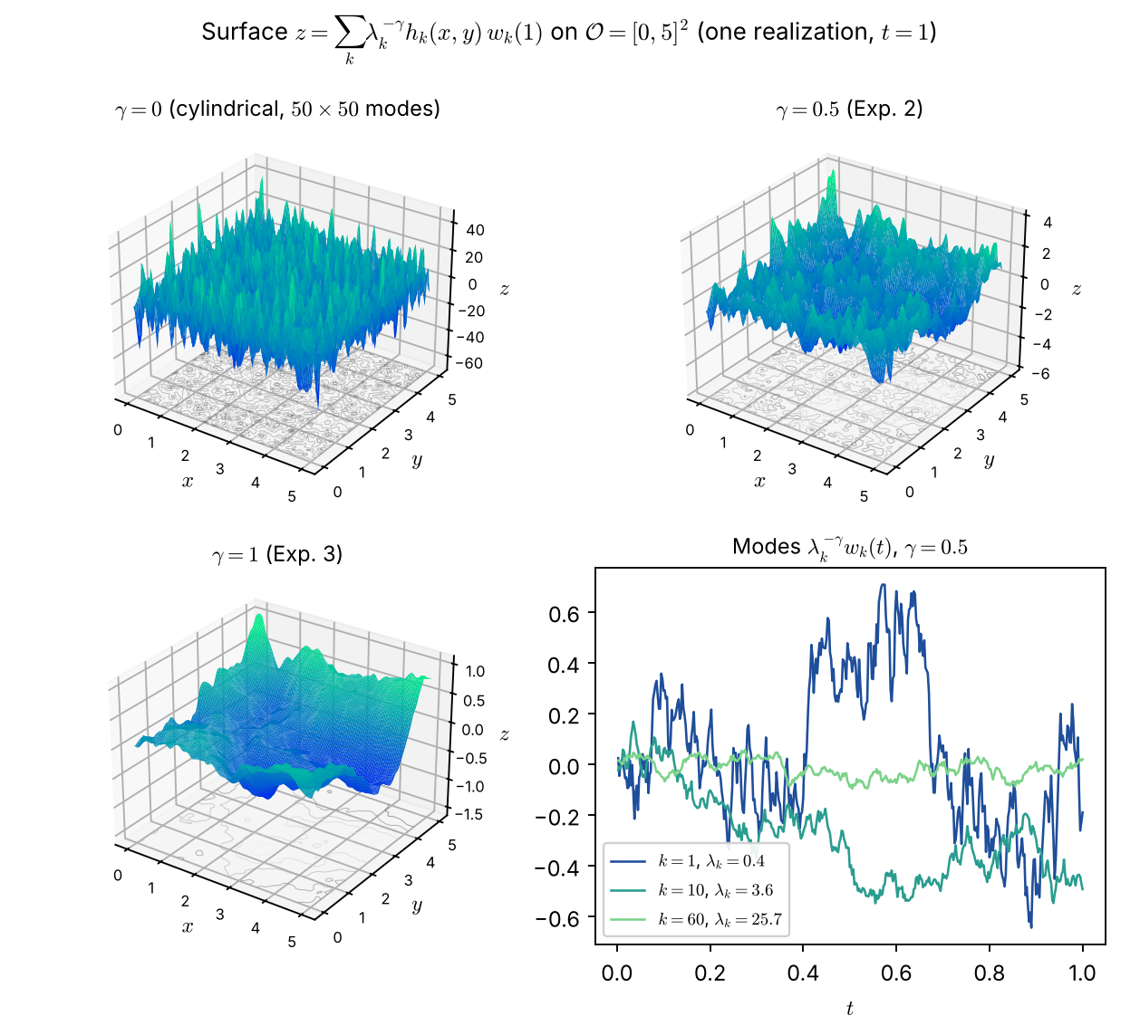
Space \((x,y)\), height \(z\) = value at \(t=1\); same \(w_k\) for all \(\gamma\), cosine basis on \(\mathcal O=[0,5]^2\), \(50\times50\) modes. Larger \(\gamma\) gives smoother noise.
Spectral Galerkin: from the SPDE to coupled SDEs
Lototsky, S. V., & Rozovsky, B. L. (2017). Stochastic Partial Differential Equations. Universitext. Springer. https://doi.org/10.1007/978-3-319-58647-2
Basis in the paper on \(\mathcal O=[0,L_1]\times[0,L_2]\), with the multi-index \(k=k(i,j)\) (\(i\) acts on \(x\), \(j\) on \(y\)), ordered by eigenvalue:
\[h_k=h_{(i,j)}=\sqrt{2-\delta_{i,0}}\sqrt{2-\delta_{j,0}}\,\cos\tfrac{\pi i x}{L_1}\cos\tfrac{\pi j y}{L_2},\qquad \lambda_k=\lambda_{(i,j)}=\pi^2\Big(\frac{i^2}{L_1^2}+\frac{j^2}{L_2^2}\Big).\]
(i) Expansion in the Neumann eigenbasis:
\[u(t,\mathbf x)=\sum_{k\in\mathbb N}u_k(t)\,h_k(\mathbf x),\]
\[u_k(t)=\big(u(t,\cdot),h_k\big)_{\mathcal H}.\]
(ii) Each mode is an OU-type process, coupled through the advection (Lototsky & Rozovsky, 2017):
\[\begin{aligned}du_k&=-\beta\lambda_k u_k\,dt-\theta\sum_{j\in\mathbb N}u_j\,v_{j,k}\,dt\\&\quad+\sigma\lambda_k^{-\gamma}\,dw_k(t),\end{aligned}\]
\[v_{j,k}:=\big(\bar{\mathbf v}\cdot\nabla h_j,\,h_k\big)_{\mathcal H}.\]
(iii) Truncated system. Keeping \(N\) modes, the column vector
\[U^N(t)=\big(u^N_1(t),\dots,u^N_N(t)\big)^{\top}\]
solves the linear OU system
\[\color{#0077b6}{dU^N=\big(-\beta\Lambda^N-\theta A^N\big)\,U^N\,dt+\sigma B^N\,dW^N(t)}\]
with
\[(\Lambda^N)_{k,k}=\lambda_k,\qquad (B^N)_{k,k}=\lambda_k^{-\gamma},\]
\[(A^N)_{k,j}=v_{j,k}\ \text{(dense)},\qquad W^N=(w_1,\dots,w_N)^{\top}.\]
Skew-symmetry of the advection matrix
Lemma 1 (skew-symmetry). If \(\nabla\cdot\bar{\mathbf v}=0\) in \(\mathcal O\) and \(\bar{\mathbf v}\cdot\mathbf n=0\) on \(\partial\mathcal O\), then
\[A^N=-\big(A^N\big)^{\top},\qquad (A^N)_{k,j}=v_{j,k}=\big(\bar{\mathbf v}\cdot\nabla h_j,\,h_k\big)_{\mathcal H}.\]
(i) Advection adds rotation, never energy: \(U^{\top}A^NU=0\), hence
\[\big\|e^{-(\beta\Lambda^N+\theta A^N)t}\big\|\le e^{-\beta\lambda_1 t},\qquad t\ge0 .\]
(ii) Numerically: \(v_{j,k}\) is computed in closed form, so \(A^N\) stays skew-symmetric to machine precision and \(\widehat\theta\) is not biased.
Convergence of the Galerkin approximation
Main obstacle: the projection \(P_N\) does not commute with \(\bar{\mathbf v}\cdot\nabla\). Split the error into tail and Galerkin parts:
e^N:=u-u^N=\underbrace{(I-P_N)u}_{\delta^N\ \text{(tail)}}+\underbrace{P_Nu-u^N}_{\rho^N\ \text{(Galerkin)}}
P_N u:=\sum_{k=1}^{N}(u,h_k)_{\mathcal H}\,h_k
The two errors
Tail \(\delta^N=(I-P_N)u\): unresolved modes \(k>N\), with \(\mathbb E\|\delta^N\|^2\lesssim\lambda_N^{-2\gamma}\).
Galerkin \(\rho^N=P_Nu-u^N\), where \(u^N\) solves the truncated OU system (10): error due only to the dropped coupling with the tail.
Theorem 1 (strong \(L^2\)-convergence rate).
\sup_{t\in[0,T]}\mathbb E\|u(t)-u^N(t)\|_{\mathcal H}^2\le C\,\lambda_N^{-2\gamma}
=\mathrm{O}\big(N^{-4\gamma/d}\big)
by Weyl's law \(\lambda_N\sim\varpi N^{2/d}\). In 2D: \(\mathrm{O}(N^{-2\gamma})\).
\(C=C(\beta,\theta,\sigma,\|\bar{\mathbf v}\|_\infty,T)\) is independent of \(N\).
Implementation on a rectangle: exact advection matrix
Neumann cosine basis on \([0,L_1]\times[0,L_2]\):
h_{(i,j)}(x,y)=\sqrt{2-\delta_{i,0}}\,\cos\!\Big(\pi i\frac{x}{L_1}\Big)\sqrt{2-\delta_{j,0}}\,\cos\!\Big(\pi j\frac{y}{L_2}\Big)
\lambda_{(i,j)}=\frac{\pi^2 i^2}{L_1^2}+\frac{\pi^2 j^2}{L_2^2},\qquad i,j\in\mathbb N\cup\{0\}
Velocity from a stream function, \(\psi|_{\partial\mathcal O}\equiv0\):
\begin{aligned}\bar{\mathbf v}&=(v_1,v_2)=(-\partial_y\psi,\,\partial_x\psi),\\ \psi(x,y)&=\sum_{r,s\in\mathbb N} \alpha_{(r,s)}\,\psi_{(r,s)}(x,y),\\ \psi_{(r,s)}(x,y)&=2\sin\Big(\pi r\frac{x}{L_1}\Big)\sin\Big(\pi s\frac{y}{L_2}\Big),\qquad r,s\in\mathbb N,\\ \alpha_{(r,s)}&=\frac{1}{L_1L_2}\int_0^{L_2}\!\!\int_0^{L_1}\psi(x,y)\,\psi_{(r,s)}(x,y)\,dx\,dy\\[6pt] &\small\text{In the experiments: } \psi=\psi_{(1,1)},\ \text{i.e. } \alpha_{(1,1)}=1,\ \alpha_{(r,s)}=0 \text{ otherwise.}\end{aligned}
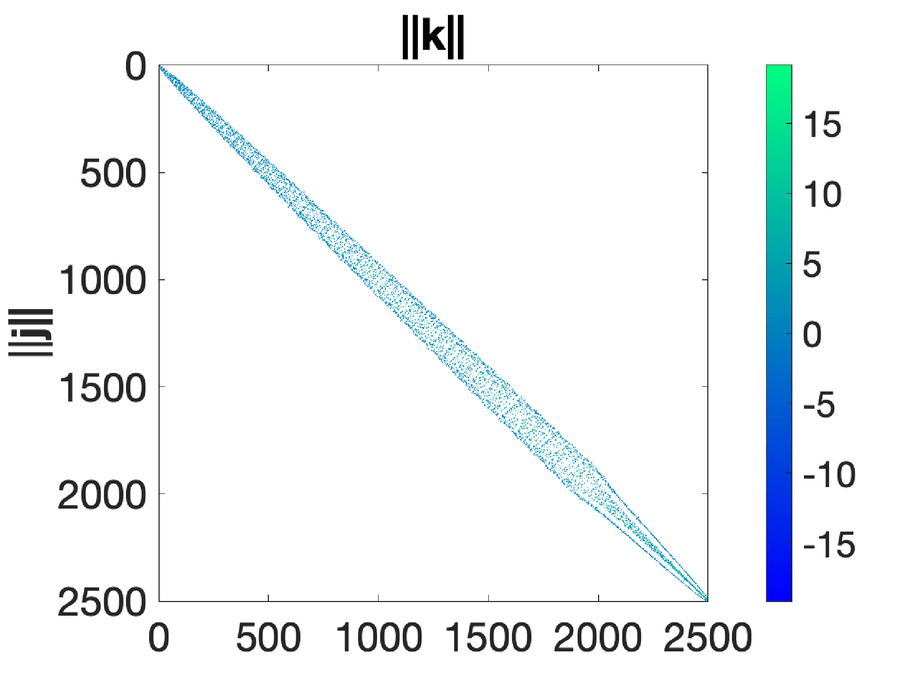
Non-zero entries of \(A_{(1,1)}\) (\(50\times50\) modes, ordered by \(\|\mathbf k\|=\sqrt{i^2+j^2}\)): banded, sparse.
{\color{#162D54}\begin{aligned}&\textbf{Advection matrix:}\quad (A^N)_{(k,l),(i,j)}=v_{(i,j),(k,l)}=\big(\bar{\mathbf v}\cdot\nabla h_{(i,j)},\,h_{(k,l)}\big)_{\mathcal H}=-(A^N)_{(i,j),(k,l)},\\ &A^N=\sum_{r,s\in\mathbb N}\alpha_{(r,s)}\,A_{(r,s)},\quad A_{(r,s)}:=A^N\ \text{for}\ \psi=\psi_{(r,s)}\ \ (\text{here } A^N=A_{(1,1)}).\end{aligned}}
Experiment 1: deterministic validation (\(\sigma=0\))
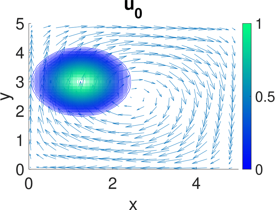
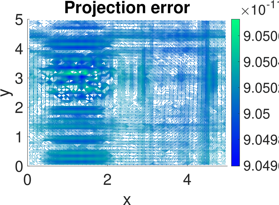
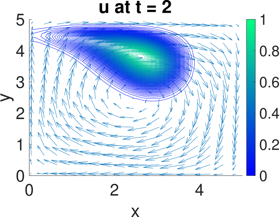
(a) \(\bar{\mathbf v}=(v_1,v_2)\) for \((r,s)=(1,1)\) and \(u_0\)
(b) Projection error of \(u_0\): \(\sim10^{-11}\)
(c) Solution at \(t=2\), \(\theta=1,\ \beta=0.01\)
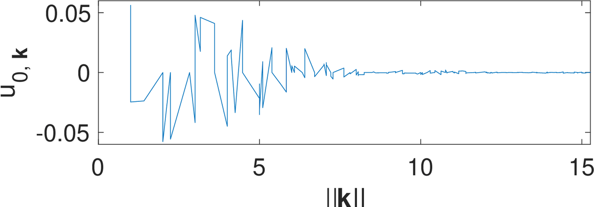
\(\mathcal O=[0,5]^2\), \(N_x\times N_y=50\times50\) modes, \(\Delta t=4\times10^{-3}\).
Method: spectral Galerkin scheme with the exact skew-symmetric \(A_{(1,1)}\), implemented in MATLAB.
(d) Spectral coefficients \(u_{0,\mathbf k}\) vs. \(\|\mathbf k\|\): energy in the first ~200 modes
Experiment 2: effect of the additive noise
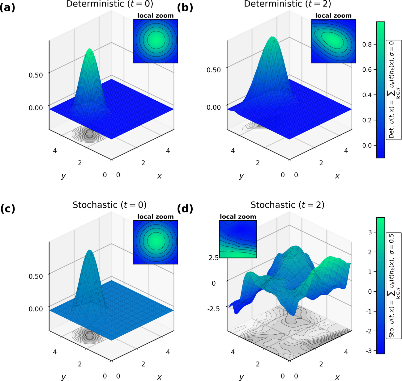
Same initial condition; deterministic (top) vs stochastic (bottom).
\(\sigma=0.5\), \(\theta=0.09\), \(\beta=0.01\), \(\gamma=0.5\); \(M=40\,000\) steps of size \(\Delta t=5\times10^{-5}\).
Data for inference: one realization of the coupled modes \(U^N(t)\).
Step 1: noise intensity from quadratic variation
\(\sigma\) enters only through the diffusion term, so it decouples from the drift:
\langle u_k,u_k\rangle_t:=\sum_{i=1}^{n^*}\big[u_k(t_i)-u_k(t_{i-1})\big]^2,\qquad \langle u_k,u_k\rangle_T=\sigma^2\lambda_k^{-2\gamma}\,T
\widehat{\sigma}^{2}:=\frac{1}{NT}\sum_{k=1}^{N}\lambda_k^{2\gamma}\,\langle u_k,u_k\rangle_T\ \xrightarrow{\text{a.s.}}\ \sigma^2
- Unbiased, strongly consistent and asymptotically normal (mesh \(\to0\), \(N\) large).
- In the simulations it is by far the most precise estimator.
- From here on \(\sigma\) is treated as known: focus on the drift parameters \(\beta,\theta\).
Step 2: likelihood via Girsanov
Theorem (Girsanov; Liptser & Shiryaev, 2001). Let \(X\) and \(Y\) be the solutions of
\[dX_t=a(t,X)\,dt+b\,dW_t,\qquad dY_t=b\,dW_t,\qquad X_0=Y_0,\]
with \(b\) invertible and
\[\int_0^T\big|b^{-1}a(t,X)\big|^2dt<\infty\quad\text{a.s.}\]
Then \(\mathbb P_X\sim\mathbb P_Y\) and
\[\begin{aligned}\frac{d\mathbb P_X}{d\mathbb P_Y}(X)=\exp\Big(&\int_0^T a^{\top}(bb^{\top})^{-1}\,dX_t\\&-\frac12\int_0^T a^{\top}(bb^{\top})^{-1}a\,dt\Big).\end{aligned}\]
Applied to the first \(N\) Galerkin modes, \(X=(u_1,\dots,u_N)\):
\[du_k=-\Big(\beta\lambda_k u_k+\theta\sum_{j=1}^N u_j\,v_{j,k}\Big)dt+\sigma\lambda_k^{-\gamma}\,dw_k,\]
so \(b=\sigma\,\mathrm{diag}(\lambda_k^{-\gamma})\), and \(\mathbb P_0\) is the law with \(\beta=\theta=0\).
The log-likelihood \(l:=\log L\) is quadratic in \((\beta,\theta)\):
\begin{aligned} L(\beta,\theta)&:=\frac{d\mathbb P_{\beta,\theta}}{d\mathbb P_0},\\[2pt] l(\beta,\theta)&=-\frac{\beta}{\sigma^2}J_1-\frac{\theta}{\sigma^2}J_2\\ &\quad-\frac{1}{2\sigma^2}\Big[\beta^2 I_1+2\beta\theta\,\mathcal J_{1,2;1}+\theta^2\mathcal J_{0,2;2}\Big]. \end{aligned}
All quantities are computable from the observed Fourier coefficients; the advection enters only through \(\sum_j u_j\,v_{j,k}\).
Liptser, R. S., & Shiryaev, A. N. (2001). Statistics of Random Processes I: General Theory (2nd ed., Ch. 7). Springer. https://doi.org/10.1007/978-3-662-13043-8
I_1:=\sum_{k=1}^N\lambda_k^{2+2\gamma}\int_0^T u_k^2(t)\,dt,
J_1:=\sum_{k=1}^N\lambda_k^{1+2\gamma}\int_0^T u_k(t)\,du_k(t),
J_2:=\sum_{k=1}^N\lambda_k^{2\gamma}\int_0^T\Big[\sum_{j=1}^N u_j(t)\,v_{j,k}\Big]du_k(t),
\mathcal J_{p,q;r}:=\sum_{k=1}^N\lambda_k^{p+q\gamma}\int_0^T[u_k(t)]^{2-r}\Big[\sum_{j=1}^N u_j(t)\,v_{j,k}\Big]^r dt
Closed-form maximum likelihood estimators
\begin{aligned}\widehat{\beta}_{N,T}&=-\frac{\mathcal J_{0,2;2}\,J_1-\mathcal J_{1,2;1}\,J_2}{\Delta_{N,T}},\\[6pt] \widehat{\theta}_{N,T}&=\frac{\mathcal J_{1,2;1}\,J_1-I_1\,J_2}{\Delta_{N,T}}.\end{aligned}
Lemma 2. \(I_1\,\mathcal J_{0,2;2}-\big(\mathcal J_{1,2;1}\big)^2>0\) almost surely, so the MLE is well defined.
The score equations are linear in \((\beta,\theta)\): the estimator is a \(2\times2\) linear solve, no optimisation.
I_1:=\sum_{k=1}^N\lambda_k^{2+2\gamma}\int_0^T u_k^2(t)\,dt,
J_1:=\sum_{k=1}^N\lambda_k^{1+2\gamma}\int_0^T u_k(t)\,du_k(t),
J_2:=\sum_{k=1}^N\lambda_k^{2\gamma}\int_0^T\Big[\sum_{j=1}^N u_j(t)\,v_{j,k}\Big]du_k(t),
\mathcal J_{p,q;r}:=\sum_{k=1}^N\lambda_k^{p+q\gamma}\int_0^T[u_k(t)]^{2-r}\Big[\sum_{j=1}^N u_j(t)\,v_{j,k}\Big]^r dt,
\Delta_{N,T}:=I_1\,\mathcal J_{0,2;2}-\big(\mathcal J_{1,2;1}\big)^2.
Fisher information: how fast do we learn?
\mathcal I_{N,T}(\beta,\theta)=\frac{1}{\sigma^2}\,\mathbb E_{\beta,\theta}\begin{pmatrix}I_1&\mathcal J_{1,2;1}\\\mathcal J_{1,2;1}&\mathcal J_{0,2;2}\end{pmatrix}=:\begin{pmatrix}\mathcal I_{\beta\beta}&\mathcal I_{\beta\theta}\\\mathcal I_{\theta\beta}&\mathcal I_{\theta\theta}\end{pmatrix}
\mathcal I_{N,T}\sim\begin{pmatrix}\mathrm{O}\big(T\,N^{1+2/d}\big)&0\\0&\mathrm{O}(T\,N)\end{pmatrix}
Both parameters become identifiable as \(N,T\to\infty\); \(\beta\) is learned faster than \(\theta\) (extra factor \(N^{2/d}\)): this is exactly what the Monte Carlo study shows.
Reading the rates
(i) \(\mathcal I_{\beta\beta}\sim T N^{1+2/d}\): each mode adds \(\approx T\lambda_k\); Weyl's law sums to \(N^{1+2/d}\).
(ii) \(\mathcal I_{\theta\theta}\sim T N\): banded \(A\) + Parseval, each mode adds \(\mathrm{O}(T)\).
(iii) Zero off-diagonal: skew-symmetry of \(A\) decouples \(\beta\) and \(\theta\).
(iv) Std. errors \(\approx\mathcal I^{-1/2}\): \(\beta\) is learned faster by a factor \(N^{1/d}\).
Asymptotic theory
Theorem 2 (consistency) \((N,T\to\infty)\)
\widehat{\beta}_{N,T}\xrightarrow{\ \mathbb P\ }\beta_0,\qquad \widehat{\theta}_{N,T}\xrightarrow{\ \mathbb P\ }\theta_0.
Theorem 3 (asymptotic normality)
\begin{aligned}\sqrt{\mathcal I_{\beta\beta}}\,\big(\widehat{\beta}_{N,T}-\beta_0\big)&\xrightarrow{d}\mathcal N(0,1),\\ \sqrt{\mathcal I_{\theta\theta}}\,\big(\widehat{\theta}_{N,T}-\theta_0\big)&\xrightarrow{d}\mathcal N(0,1).\end{aligned}
Full modal coupling does not destroy the classical picture: consistent and asymptotically Gaussian MLEs, with rates given by the Fisher information.
Experiment 3: estimators along one sample path
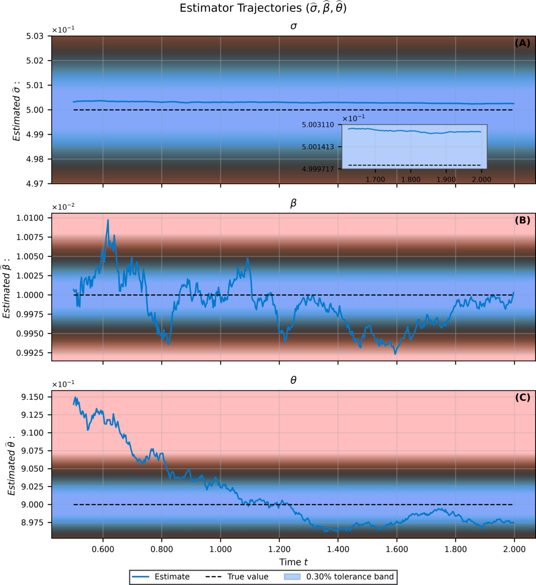
- \(\widehat\sigma,\widehat\beta,\widehat\theta\) as the horizon \(T\) grows; dashed: true values.
- \(N_x=N_y=20\) modes.
- \(\widehat\sigma\) stabilises almost immediately.
- \(\widehat\beta\), \(\widehat\theta\): longer transient; \(\widehat\theta\) fluctuates more (it lives on the modal interactions).
- Trajectories enter and stay in the low-relative-error band.
Monte Carlo: 1000 replications per setting
Experimental setup. True values: \({\color{#1B6B3A}\beta=0.1},\ {\color{#1B6B3A}\theta=0.1},\ {\color{#1B6B3A}\sigma=1.0}\)
Spatial modes: \(N_x=N_y=20\)
\(M\): number of time-integration steps of size \({\color{#0077B6}\Delta t}\) with the Milstein method
| \(M=1000\) | \(5000\) | \(20\,000\) | \(50\,000\) | ||
|---|---|---|---|---|---|
| \({\color{#0077B6}\Delta t=10^{-7}}\) | \(\widehat\beta\) | 0.0983 (0.0224) | 0.0997 (0.0098) | 0.1000 (0.0051) | 0.1000 (0.0033) |
| \(\widehat\theta\) | 0.1078 (0.4570) | 0.1019 (0.1460) | 0.1048 (0.1041) | 0.0999 (0.0655) | |
| \({\color{#0077B6}\Delta t=10^{-5}}\) | \(\widehat\beta\) | 0.0999 (0.0024) | 0.1001 (0.0014) | 0.1001 (0.0012) | 0.1000 (0.0011) |
| \(\widehat\theta\) | 0.0998 (0.0497) | 0.0989 (0.0263) | 0.1002 (0.0209) | 0.1001 (0.0198) | |
| \({\color{#0077B6}\Delta t=10^{-4}}\) | \(\widehat\beta\) | 0.1001 (0.0012) | 0.1002 (0.0011) | 0.1001 (0.0010) | 0.1001 (0.0008) |
| \(\widehat\theta\) | 0.0999 (0.0233) | 0.0999 (0.0186) | 0.0991 (0.0148) | 0.0996 (0.0104) | |
| Run Avg. time (s) | 0.07 | 0.33 | 1.32 | 3.59 | |
Table. Mean of the estimates over 1000 replications, with the empirical standard deviation (s.d.) in orange.
- \(\widehat\beta\): maximum likelihood estimator of the diffusion
- \(\widehat\theta\): maximum likelihood estimator of the advection coupling
- \(M\): number of time integration steps
- \({\color{#0077B6}\Delta t}\): time step between observations
- Run Avg. time: mean computing time per estimate, in seconds
Empirical distributions: asymptotic normality
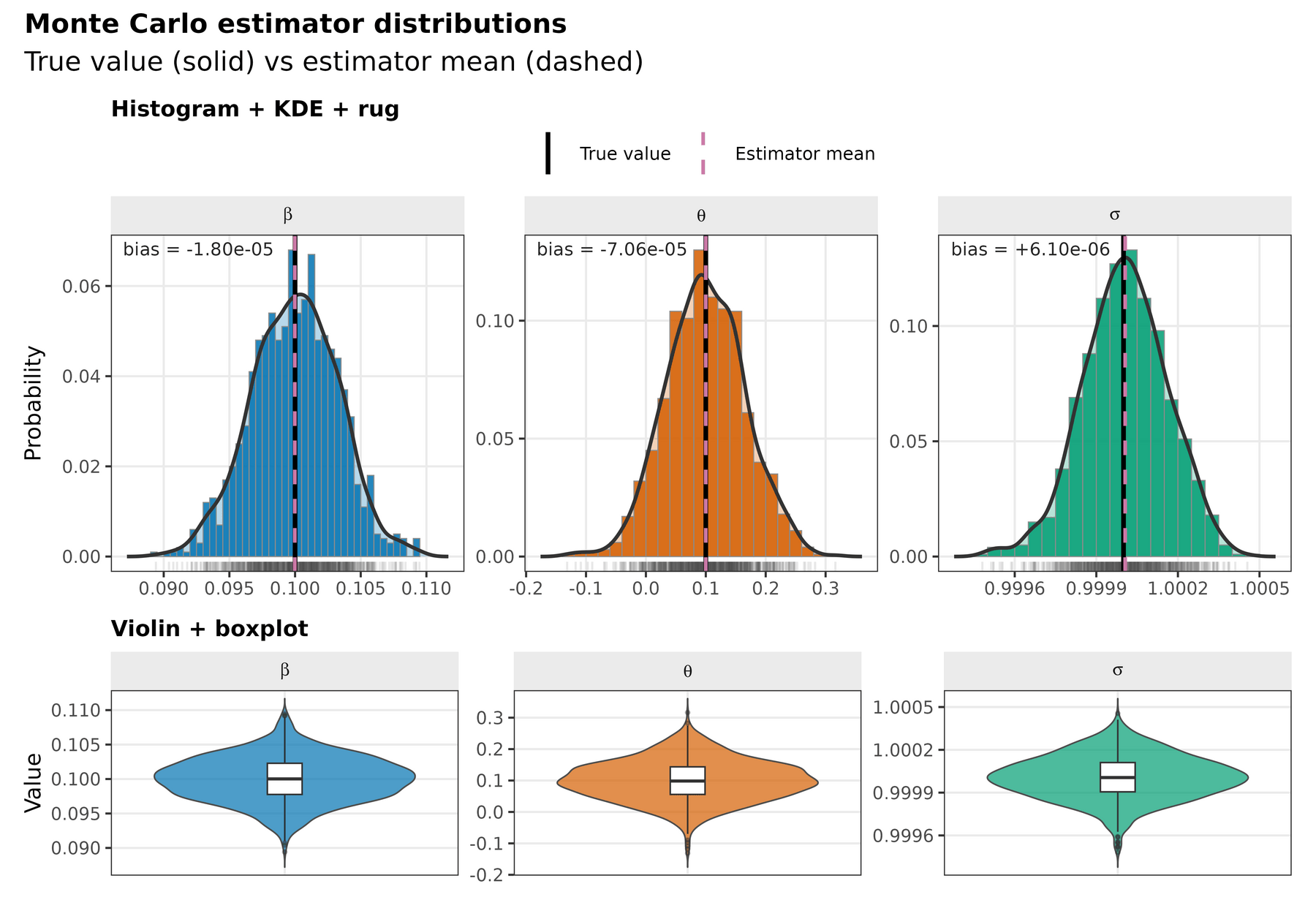
- 1000 replications, \(M=50\,000\), \(\Delta t=10^{-7}\).
- Symmetric, centred at the truth.
- \(\widehat\beta\): close to Gaussian.
- \(\widehat\theta\): larger spread.
- \(\widehat\sigma\): sharply concentrated.
How many modes do we need?
Experimental setup. True values: \({\color{#1B6B3A}\beta=0.1},\ {\color{#1B6B3A}\theta=0.1},\ {\color{#1B6B3A}\sigma=1.0}\)
\(M=50\,000\) time-integration steps of size \({\color{#0077B6}\Delta t=10^{-7}}\) with the Milstein method
Spatial modes varied: \(N_x=N_y\in\{5,10,15,20\}\)
| \(N_x=N_y\) | \(5\) | \(10\) | \(15\) | \(20\) |
|---|---|---|---|---|
| \(\widehat\beta\) | 0.1169 (0.3098) | 0.1016 (0.0319) | 0.1000 (0.0083) | 0.1000 (0.0033) |
| \(\widehat\theta\) | 0.0233 (2.2634) | 0.0972 (0.2691) | 0.0994 (0.1166) | 0.0999 (0.0655) |
| \(\widehat\sigma\) | 1.0000 (0.0007) | 1.0000 (0.0003) | 1.0000 (0.0002) | 1.0000 (0.0002) |
| Run Avg. time (s) | 0.04 | 0.29 | 1.18 | 3.59 |
Table. Mean of the estimates over 1000 replications, with the empirical standard deviation (s.d.) in orange.
- \(\widehat\beta\): maximum likelihood estimator of the diffusion
- \(\widehat\theta\): maximum likelihood estimator of the advection coupling
- \(\widehat\sigma\): estimator of the noise intensity
- \(N_x,N_y\): number of Fourier modes in each direction
- Run Avg. time: mean computing time per estimate, in seconds
Conclusions and outlook
Contributions
- Explicit MLEs for \(\beta,\theta\) under full modal coupling.
- Galerkin rate \(\mathrm{O}(N^{-4\gamma/d})\) despite non-commuting \(P_N\).
- Consistency and asymptotic normality (Malliavin–Stein) as \(N,T\to\infty\).
- Exact skew-symmetric advection matrix: efficient and bias-free.
Next steps
- Multiplicative noise for positive concentrations.
- Time-dependent velocity fields \(\bar{\mathbf v}(t,x)\).
- Cheaper truncation / localised estimation for large \(N\).
- Sargassum: logistic growth \(ru(1-u/K)\), calibration with satellite/drifter data, uncertainty bands for arrivals.
Diligence: responsible use of AI
4D AI Fluency framework (Dakan & Feller, 2025): Delegation · Description · Discernment · Diligence, i.e. taking responsibility for what we do with AI and how we do it.
Creation diligence. AI systems were chosen deliberately, each one for a defined task (table).
Transparency diligence. The role of AI in this work is disclosed on this slide and in the repository.
Deployment diligence. All AI-generated code was reviewed and validated by the authors: deterministic test (Exp. 1), Monte Carlo recovery of the true parameters, and skew-symmetry of \(A^N\) to machine precision. We stand behind the results.
AI tools used
| Tool | Version / model | Role |
|---|---|---|
| Claude Code | v2.1.305; model claude-opus-5-5 | Fortran and Python code generation |
| OpenAI Codex | GPT-5.6 | Fortran and Python code generation |
| GitHub Copilot | Copilot CLI v1.0.83 | GitHub management of the report |
| Claude (Cowork, in Chrome) | model claude-opus-5-5 | Slide layout and formatting |
Authors (responsible for all content): Saúl Díaz-Infante (SECIHTI – Universidad de Sonora), Fernando Baltazar-Larios (UNAM), Francisco Delgado-Vences (UAB, Barcelona), Gerardo Hernández-Dueñas (IM-UNAM, Juriquilla).
Dakan, R., & Feller, J. (2025). The 4Ds: AI Fluency Framework. Anthropic. CC BY-NC-SA 4.0. https://www-cdn.anthropic.com/34612aacbf37f6aa12140fc0a1aa216b63263aac.pdf. Tool versions as of October 2026.
Slides and code
These slides
slides.com/sauldiazinfantevelasco
Thank you! · saul.diazinfante@unison.mx
59 Congreso Nacional de la Sociedad Matemática Mexicana:SMN
By Saul Diaz Infante Velasco
59 Congreso Nacional de la Sociedad Matemática Mexicana:SMN
Discover innovative approaches in numerical simulation and maximum likelihood estimation for stochastic convection-diffusion equations, presented by Saúl Diaz Infante Velasco at the 59th National Congress of the Mexican Mathematical Society. Exciting insights await!