
















































![Delta_K^gzip,(d) = E[ CD(A1,B1) - 1/2 {CD(A1,A2) + CD(B1,B2)} ]](https://s3.amazonaws.com/media-p.slid.es/uploads/194679/images/13081291/image49.png)


















Ishanu Chattopadhyay PRO
ML | Data Science Biomedical Informatics | Social Science | Assistant Professor
PI: Ishanu Chattopadhyay, PhD
Assistant Professor of Biomedical Informatics & Computer Science
University of Kentucky
DARPA-EA-25-02-05-MAGICS-PA-025
HR0011-26-3-E016
May 2026For public dissemination
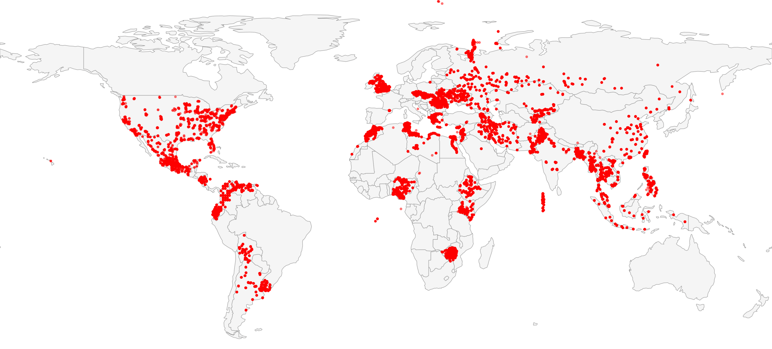
GSS
Eurobarometer
Afrobarometer
WVS
1. Large Science Models: Latent dependency non-parametric inference model working code (https://github.com/zeroknowledgediscovery/quasinet)
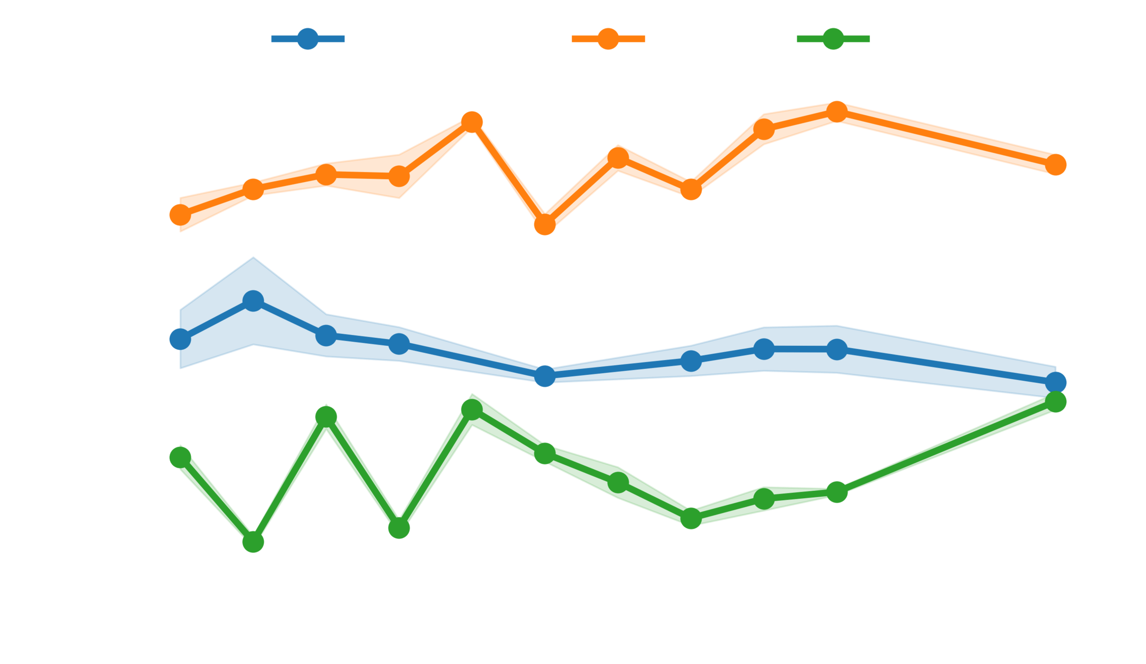
2. Extensive out-of-sample validation of response reconstruction showing substantial improvement over LLM based survey models (Fig 2)
Fig. 1
Fig. 2
LLM model: GPT 5.4
Baseline: independent generation
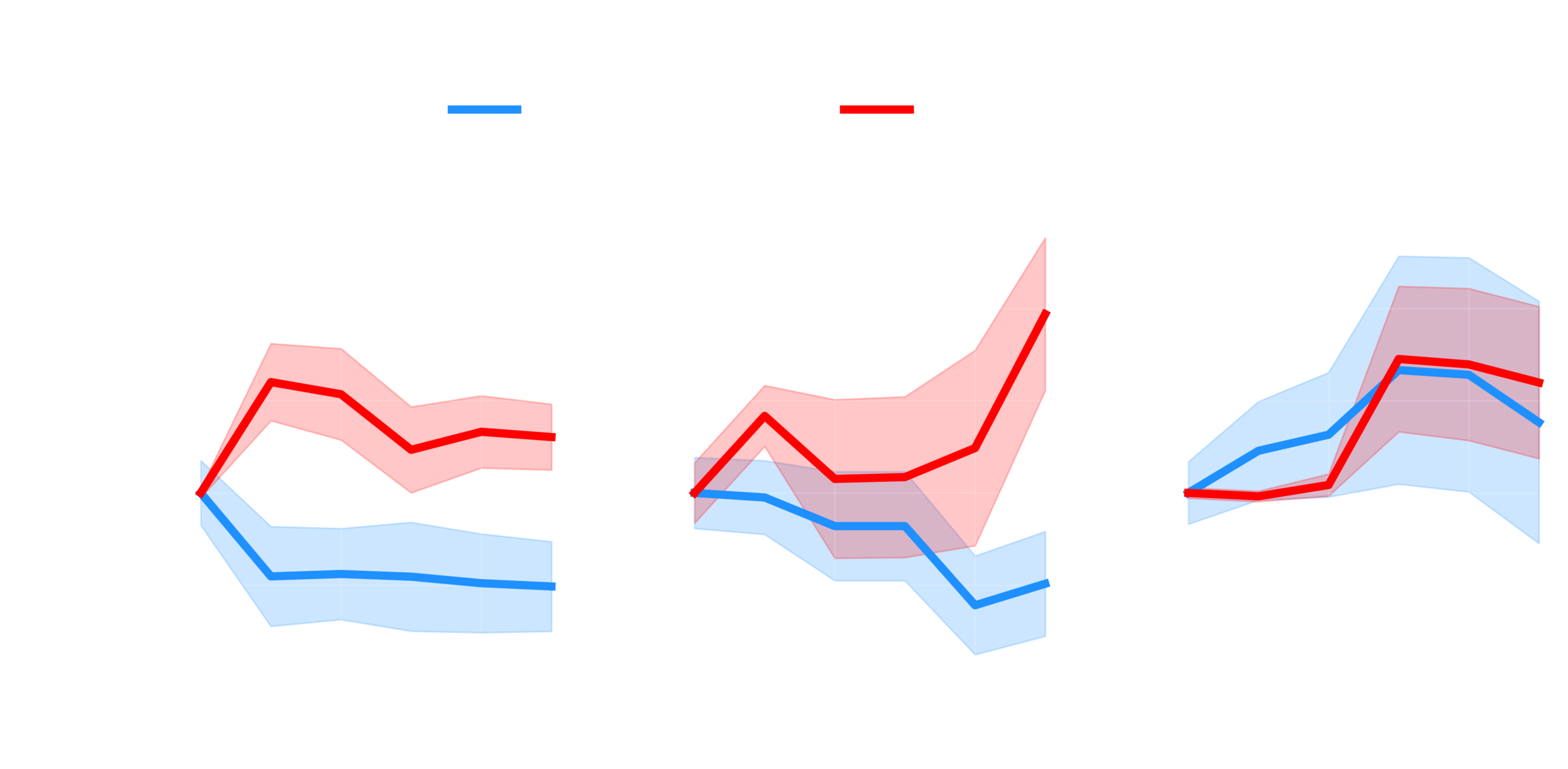
Fig. 3
3. Digital Twin Anchored Generation (DTAG) framework code in beta testing. Allowing a LLM semantic layer to access LSM models stratified by time, geolocation and demographics to make it possible to have human "conversations" with persona without hallucinations.
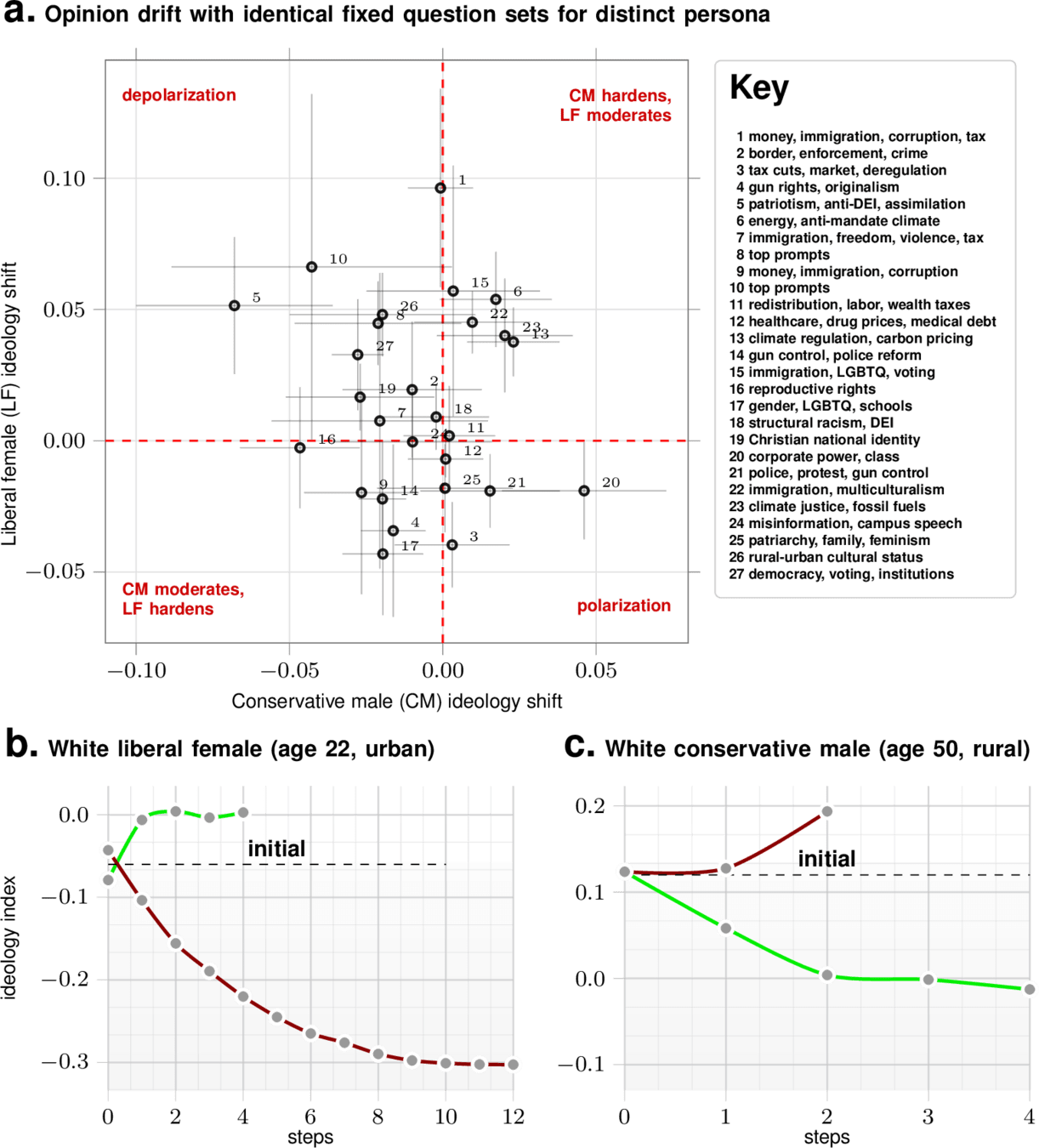
3. With DTAG, Targeted question sequences being investigated to drive opinion changes (Fig.3)
4. D. Yang, J. Evans and I. Chattopadhyay, “The Fabric of Opinion: How Interdependent Attitudes Constrain Worldviews, Predict Behavior, and Evolve Over Time", Nature Human Behavior, Under Review
Planned Abstract Submission:
Accepted Paper:
K. Wu, F. Li and I. Chattopadhyay, "Emergenet: A Digital Twin of Influenza A Evolution for Vaccine Strain Forecasting and Emergence Risk Assessment", Military Medicine, In Press
“Exposure to opposing views on social media can increase political polarization” by Christopher A. Bail et al., published in PNAS in September 2018 (Vol. 115, No. 37, pp. 9216–9221; DOI: 10.1073/pnas.1804840115)
We find more general possibilities: We can make world-views go more extreme or less extreme based on the line of questions and the persona
Perturbing with opposing views made conservatives more conservative (statistically significant), liberals more liberal (not statistically significant)
LSM
Prospective validation in Human Cohorts
x
demographic filter
persona filter
P2
P1
fixed question sets
attention questions
| 1 | Kickoff Meeting: A briefing on the technical plan for the effort to include milestone schedule and path to accomplish the objectives of the agreement. | Government acceptance / Kickoff meeting briefing slides | Month 1 after award start |
| 2 | Validation plan: Detailed validation plan, including description,acquisition plan, and justification for the ground truth data, and description of the metricsand benchmarks to be used to measure performance. | Government acceptance / Technical report as described. | Month 1 |
| 3 |
Milestone Title: Dataset Acquisition and LSM Inference Technical goal: a) Dataset acquisition (10 social survey datasets acquired: GSS, ANES, CES, Eurobarometer etc) b) Infer LSM models for each dataset using 50% random samples, multiple LSMs trained with different random splits for each dataset. |
Government acceptance / Technical report detailing figure/code/data/etc. and all underlying materials generated in support of milestone, regardless of success | Month 2 |
| 4 |
Milestone Title: Masked sample reconstruction Technical goal: LSM predictive accuracy validation via censored sample reconstruction validation on out of sample data from each dataset, Demonstrate statistically significant reduction of LSM distance post reconstruction relative to post-masking. Target: Reconstruction metric error at least 50% improvement over 1) random imputation 2) median imputation |
Government acceptance / Technical report detailing figure/code/data/etc. and all underlying materials generated in support of milestone, regardless of success | Month 4 |
| 5 |
Milestone Title: Model drift sensing validation Technical goal: Demonstrate that LSM framework can reliably sense when underlying model drifts. Assess if the model drift statistic is stationary from samples drawn from the same survey wave of our datasets, and reliably indicates non-stationary drift for samples from different survey waves. Target: Model drift statistic must have statistical significance at 5% level for survey waves 5 years apart for at least GSS, CES and Eurobarometer Deliverable are detailed documentation on all 10 datasets |
Government acceptance / Technical report detailing figure/code/data/etc. and all underlying materials generated in support of milestone, regardless of success | Month 6 |
| 6 |
Milestone Title: Data sufficiency assessment capability Technical goal: Use the conservation of complexity principle to show that LSM framework can sense data deficiency and sufficiency. |
Government acceptance / Technical report detailing figure/code/data/etc. and all underlying materials generated in support of milestone, regardless of success.Analysis results on all 10 datasets | Month 8 |
| 7 |
Milestone Title: Social Theory and Competing Hypotheses Adjudication Technical goal: a) Social Theory Hypothesis Assessment: Polarization is an inevitable attractor b) Investigate the competing hypotheses that socio-economic identity vs belief proximity and latent opinion space geometry is more predictive of specific opinion / belief outcomes |
Government acceptance / Technical report detailing figure/code/data/etc. and all underlying materials generated in support of milestone, regardless of success | Month 10 |
| 8 |
Final milestone meeting and report (one month prior to award end date): The final briefing and final report should summarize all work completed on the project, highlighting accomplishments, lessons learned, unexpected outcomes, and challenges requiring further Research. Technical artifact delivery (Software release, evaluation results, source code, models, etc.) |
Government acceptance / Technical report as described.For software: Github repository with deployable code complete with example notebooks | Month 11 |
|
Milestone Title / Detailed Description |
|
Exit Criteria /Deliverable |
|
|
Milestone # |
\(\checkmark\)
\(\checkmark\)
LARGE SCIENCE MODELS · SYSTEM-LEVEL DRIFT
The Characteristic Drift Spectrum
A task-free, multiscale fingerprint of systemic organization in complex systems
Structural drift
Information drift
Kolmogorov drift
Ishanu Chattopadhyay
University of Kentucky
MOTIVATION
Why a characteristic drift spectrum?
Characteristic Drift Spectra of Complex Systems
2 / 14
Classical dataset & concept drift
Task model / classifier
Characteristic drift spectrum
depth 0
depth 1
depth 2
The question becomes: where in the hierarchy of system states does organization change, and in what way?
LARGE SCIENCE MODEL
An LSM encodes conditional organization
Characteristic Drift Spectra of Complex Systems
3 / 14
For categorical state X = (X1, …, Xp) and row population R, an LSM is a target-wise collection of conditional predictors:
For row x, the mean conditional log-persistence is
PM(x) is the average log support assigned to the observed coordinates when each coordinate is predicted from the remainder of the state.
Low persistence identifies rows that are poorly reconstructed by the dominant learned conditional organization.
LSM construction: Sizemore et al., Sci. Adv. 2024; Wu, Li & Chattopadhyay, Mil. Med. 2026.
Masked-coordinate prediction
x1
x2
x3
?
masked
⋯
xp
MAP
observed
Conditional distribution over states a ∈ Ai
INTRINSIC RESIDUAL HIERARCHY
Peeling recovers a residual hierarchy
Characteristic Drift Spectra of Complex Systems
4 / 14
⋮
a fresh LSM at every level
1
Fit and score
2
Robustly standardize lack of persistence
3
Peel and refit
At depth d, fit Md = LSM(Rd) and compute the persistence of every row under Md.
Intuition. Peeling removes the statistically dominant core and refits on the surviving low-persistence population, so organization masked at the population level becomes visible. Depth is structural, not chronological.
COORDINATES OF THE SPECTRUM
Three scalar probes at every depth
Characteristic Drift Spectra of Complex Systems
5 / 14
PROBE I
Structural drift
MEASURES
Change in MAP-normalized masked-state reconstruction support after refitting.
BUILT FROM
The MAP-normalized reconstruction score of the LSM
PROBE II
Information drift
MEASURES
Change in description length under the conditional structure learned from the data.
BUILT FROM
The data-adaptive code length induced by the LSM
PROBE III
Kolmogorov drift
MEASURES
Compression-calibrated information displacement between adjacent residual levels.
BUILT FROM
Normalized compression distance (gzip) between matched row blocks
At every depth d, the three numbers form one point of the spectrum:
PROBE I
Structural drift
Characteristic Drift Spectra of Complex Systems
6 / 14
MAP-normalized masked-state reconstruction score
uM = 1 when the observed state attains the conditional MAP support; smaller values measure its support relative to that MAP state.
With a balanced probe cloud Qd and common evaluable targets Id(x), average the change between adjacent depths:
Same probe, adjacent depths
MAP state
observed state
Intuition. Structural drift measures how the system’s learned ability to reconstruct masked coordinates changes across structural depth.
PROBE II
Information drift
Characteristic Drift Spectra of Complex Systems
7 / 14
A data-adaptive code from the learned conditional structure
Mean code length (bits) of row x when each coordinate is encoded with the LSM’s conditional predictor.
Information drift between adjacent residual levels
Both expectations use the depth-d model Md: rows of Rd+1 are coded with structure learned on Rd.
Mean code length under Md
schematic
Intuition. An LSM-based description-length probe: information displacement is measured using structure learned from the system itself.
PROBE III
Kolmogorov drift
Characteristic Drift Spectra of Complex Systems
8 / 14
At depth d, draw matched row blocks A1, A2 ⊂ Rd and B1, B2 ⊂ Rd+1. For serialized blocks a, b and compressor length C(·), the normalized compression distance is
Within-depth distances establish the intrinsic compression scale; the across-depth distance measures separation between adjacent levels:
within depth: intrinsic scale
across depth: separation
Intuition. Compression-calibrated information displacement between adjacent residual levels, measured with a general-purpose compressor rather than the learned model.
SYNTHESIS
The characteristic drift spectrum
Characteristic Drift Spectra of Complex Systems
9 / 14
At every depth d, the three numbers form
and stacking them across depth gives a depth-by-coordinate matrix:
⋮
⋮
⋮
rows: structural depth d = 0, …, D−1 columns: the three probes
A high-dimensional system is mapped to a small, ordered set of scalar probes while preserving structural depth: a task-free fingerprint that can be compared across repeated observations.
POSITIVE CONTROL
GSS: recovering a known data shift
Characteristic Drift Spectra of Complex Systems
10 / 14
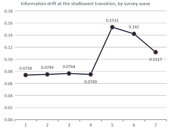
0.0750
2012–2018 mean · face-to-face
waves: 0.0738, 0.0749, 0.0764, 0.0749
0.1531
2021 · primarily web-based
≈ 2× the pre-2021 level
0.1420 → 0.1117
2022, 2024 · mixed web/face-to-face
partial return toward the earlier regime
The spectrum recovers this independently documented change in the observation process without being trained to discriminate survey years or modes.
POSITIVE CONTROL
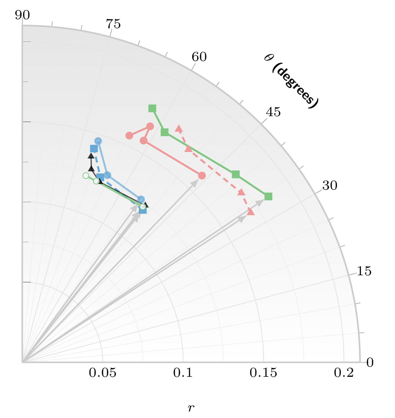
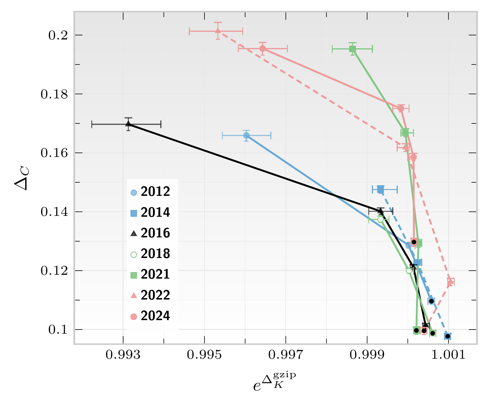
Two projections of the GSS spectrum
Characteristic Drift Spectra of Complex Systems
11 / 14
a Polar rendering of the raw (information drift, structural drift) plane. A tight 2012–2018 regime, a pronounced 2021 displacement, and partial return in 2022 and 2024.
b gzip/NCD information displacement against the Dirichlet-posterior mean of structural drift; the horizontal axis shows exp(Kolmogorov drift).
MULTISCALE COMPARISON
Spectra as fingerprints: 2018 vs 2024
Characteristic Drift Spectra of Complex Systems
12 / 14
d = 0
.0971
.0749
.00061
d = 1
.1130
.0460
.00004
d = 2
.1164
.0395
−.00090
d = 0
.1165
.1117
.00015
d = 1
.1383
.0754
−.00008
d = 2
.1472
.0794
−.00035
First three transitions; cell shading scales with value within each of the first two columns.
Reading the fingerprints
OUTLOOK
Interpretation and next steps
Characteristic Drift Spectra of Complex Systems
13 / 14
A system-level measurement object: a high-dimensional complex system mapped to a small, ordered set of scalar probes, with structural depth preserved.
Applies whenever a multivariate system admits conditional modeling without selecting a privileged response variable.
ROUTES FOR CALIBRATING THE OPERATING RANGE OF EACH COORDINATE
Matched-size refit nulls
Refit at matched sample sizes to separate real drift from refit variability.
Independent peeling rules
Recover the hierarchy with alternative peeling rules to test robustness.
Planted-change simulations
Inject known changes to map the sensitivity of each coordinate.
Alternative compressors
Test how Kolmogorov drift depends on the choice of gzip.
Observation-design controls
Separate changes in how data are collected from changes in the system.
ACKNOWLEDGMENT & REFERENCES
References
Characteristic Drift Spectra of Complex Systems
14 / 14
[1] J. G. Moreno-Torres et al., “A unifying view on dataset shift in classification,” Pattern Recognition 45(1):521–530, 2012.
[2] J. Gama et al., “A survey on concept drift adaptation,” ACM Computing Surveys 46(4), 2014.
[3] A. Gretton et al., “A kernel two-sample test,” JMLR 13:723–773, 2012.
[4] D. Lopez-Paz and M. Oquab, “Revisiting classifier two-sample tests,” ICLR, 2017.
[5] N. Sizemore et al., “A digital twin of the infant microbiome to predict neurodevelopmental deficits,” Science Advances 10(15):eadj0400, 2024.
[6] K. Wu, F. Li, and I. Chattopadhyay, “Emergenet: A digital twin of influenza A evolution for vaccine strain forecasting and emergence risk assessment,” Military Medicine, usag255, 2026.
[7] NORC at the University of Chicago, “General Social Survey 2021 codebook,” 2021.
[8] NORC, “General Social Survey 2022 codebook,” 2023.
[9] NORC, “General Social Survey 2024 codebook,” release 2, 2025.
[10] NORC, “Sequential data collection designs in the General Social Survey,” GSS Methodological Report 140, 2025.
[11] M. Li et al., “The similarity metric,” IEEE Trans. Information Theory 50(12):3250–3264, 2004.
Correspondence: ishanu_ch@uky.edu
Acknowledgment. This material is based upon work supported by the Defense Advanced Research Projects Agency (DARPA) under Agreement No. HR0011-26-3-E016. The views, opinions, and/or findings expressed are those of the authors and should not be interpreted as representing the official views or policies of the Department of Defense or the U.S. Government.
By Ishanu Chattopadhyay
DARPA-EA-25-02-05-MAGICS-PA-025 PI/PM Meeting