Robust characterisation of transient radio light curves using Gaussian process regression
Shih Ching Fu
shihching.fu@postgrad.curtin.edu.au
Supervisors:
Dr Arash Bahramian, Dr Aloke Phatak,
Dr James Miller-Jones, Dr Suman Rakshit
Light Curves
- Light curves are time series data describing the changing brightest of a source over time.
- The shape of a light curve can identify and reveal properties of the underlying object or event.
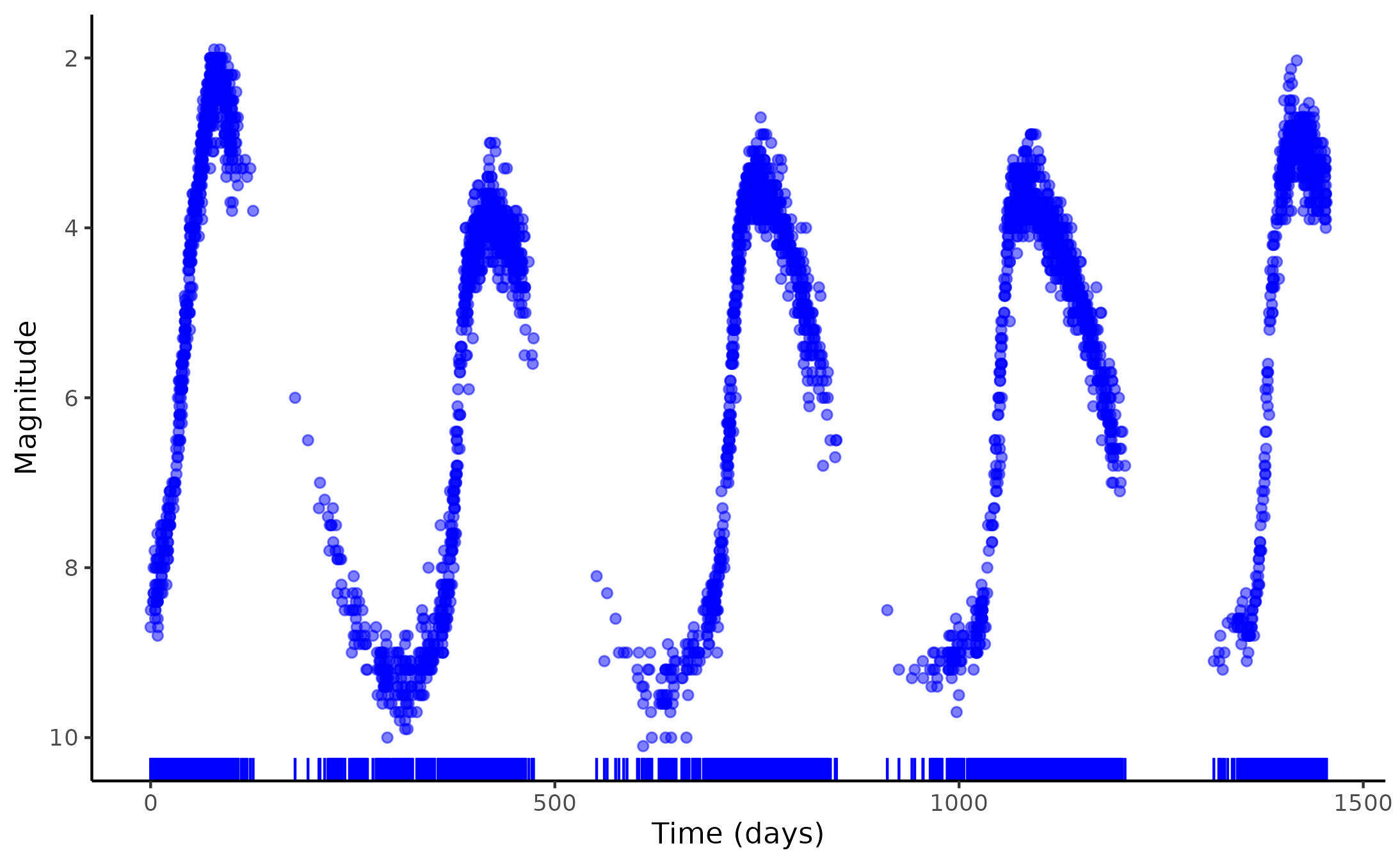
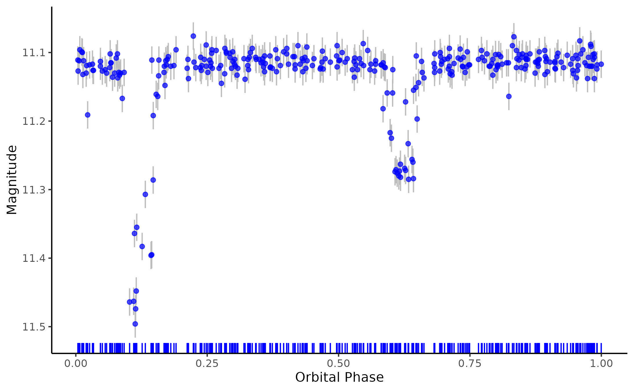
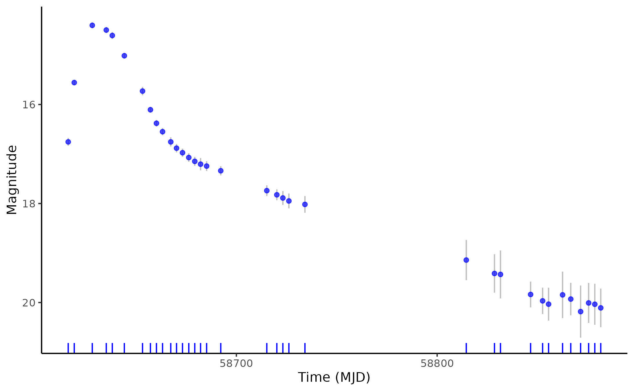
Treat the varying brightness of a source as a stochastic process
Magnitude
Magnitude
Magnitude
Time (days)
Orbital Phase
Time (MJD)
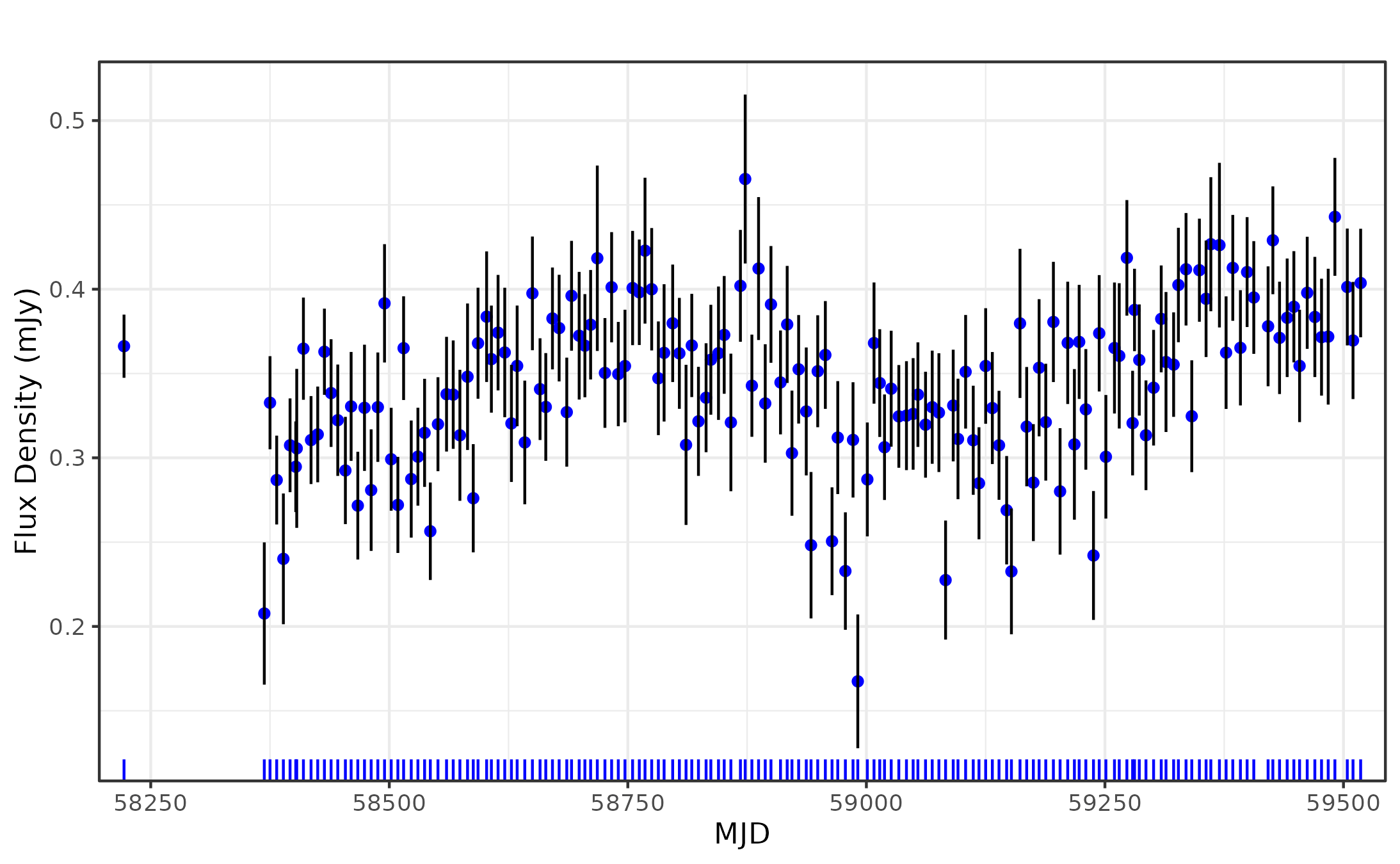
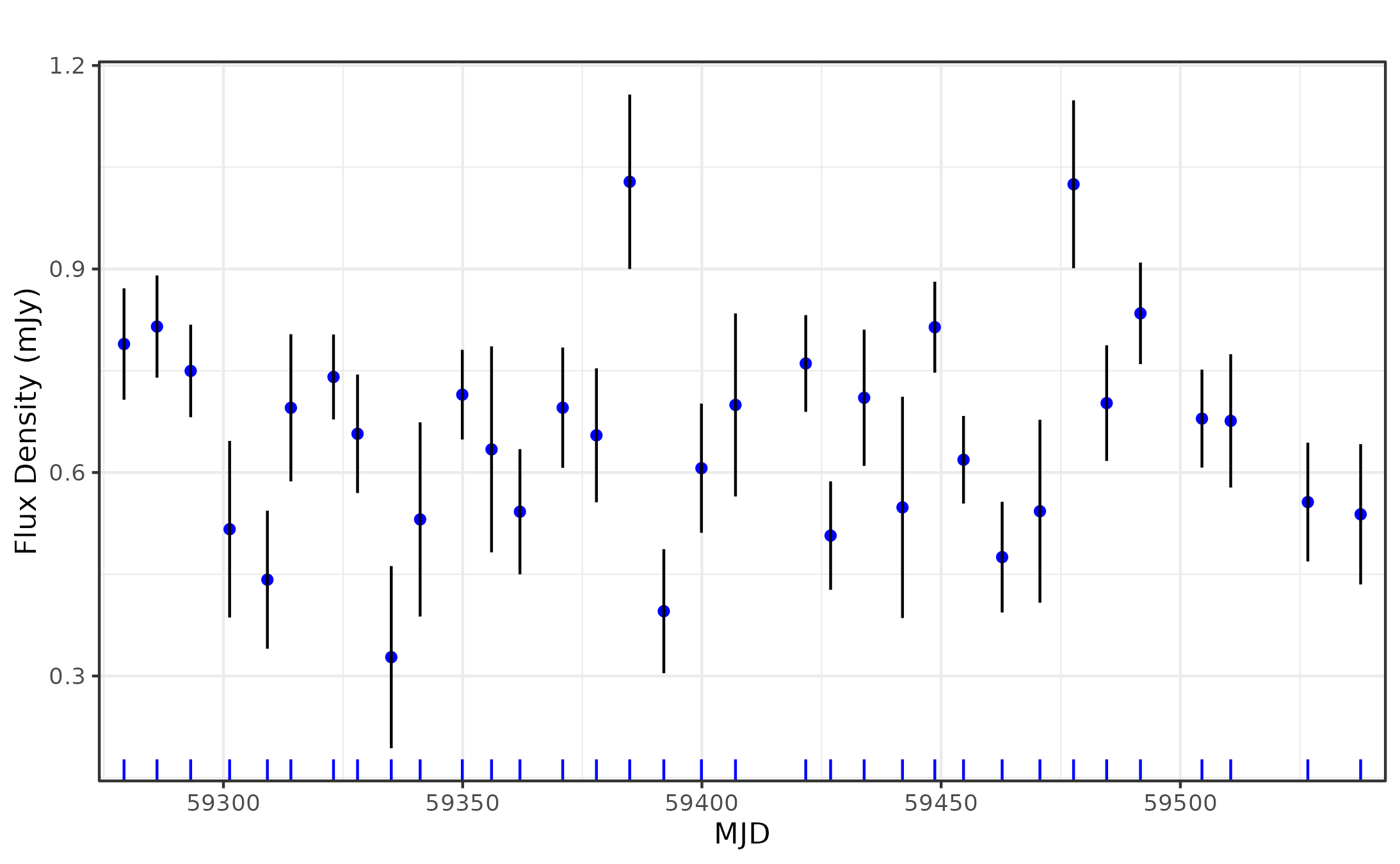
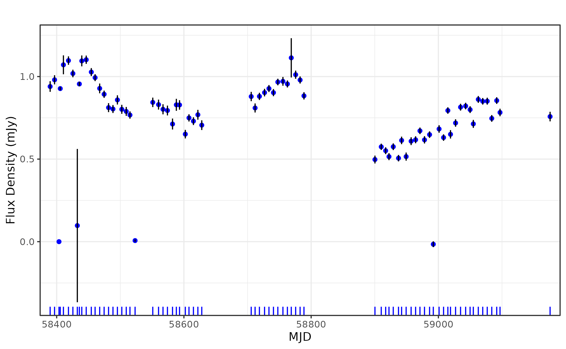
Heterogeneous Data
- Different cadences
- Sparse observations
- Uneven sampling rates
- Varying noise levels
Characterising Light Curves
- Fewer parameters
- Scales easily
- High information loss
- Many parameters
- High discriminatory power
- Overfitting
Oversimplified
Overspecified
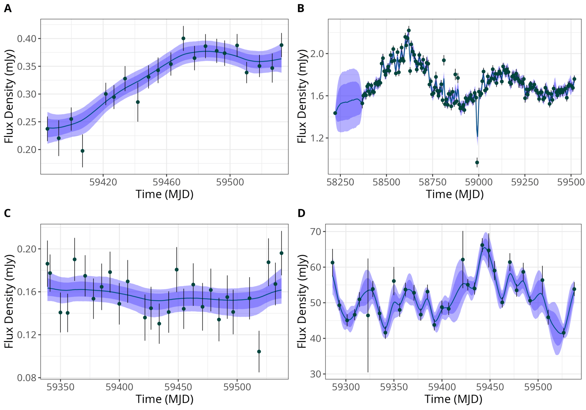
Model light curves as a Gaussian Process (GP)
Multivariate Normal
Y is a vector of n Gaussian distributed random variables.
\begin{bmatrix}
Y_1 \\
\vdots \\
Y_n
\end{bmatrix} \sim \mathcal{N}_n (\boldsymbol{\mu}, \boldsymbol{\Sigma}_{n \times n})
\boldsymbol{\Sigma}_{n \times n} =
\begin{bmatrix}
\Sigma_{11} & \dots & \Sigma_{1n} \\
\vdots & \ddots & \vdots \\
\Sigma_{n1} & \dots & \Sigma_{nn}
\end{bmatrix}
where \(\boldsymbol\mu = (\mu_1, \dots, \mu_n)\) and \(\boldsymbol{\Sigma}\) is a \(n \times n \) covariance matrix.

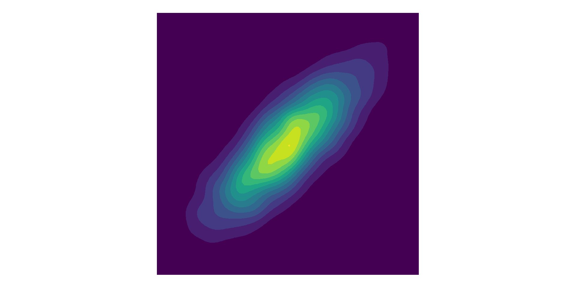
\mathbf{\Sigma} =
\begin{bmatrix}
1 & 0 \\
0 & 1
\end{bmatrix}
\mathbf{\Sigma} =
\begin{bmatrix}
1 & 0.8 \\
0.8 & 1
\end{bmatrix}
- Symmetric, positive semi-definite matrix.
- Linear combinations are also valid covariance matrices.
Gaussian Processes (GPs)
Extend multivariate Gaussian to 'infinite' dimensions.
- Mean function, \(\mu(t)\)
- Covariance or kernel function, \( \kappa(t,t') \)
\begin{bmatrix}
Y_1 \\
Y_2 \\
\vdots \\
\end{bmatrix} \sim \mathcal{GP} (\mu(t), \boldsymbol{\Sigma})
where \(\mu = \mu(t_i)\) and \( [\boldsymbol\Sigma]_{ij} = \kappa(t_i, t_j) \), for \( i,j = 1, 2, \dots \)
Rather than specify a fixed covariance matrix with fixed dimensions, compute covariances using the kernel function.
Kernel Functions
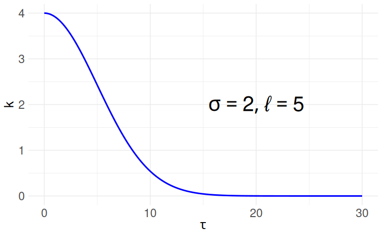
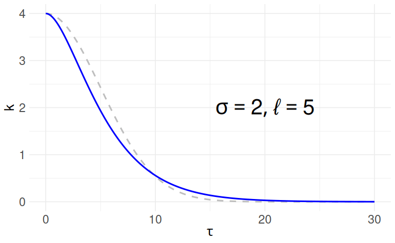
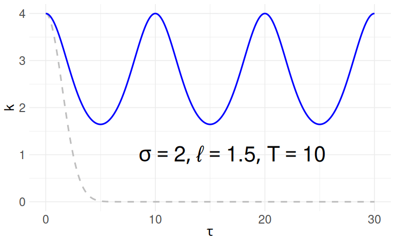
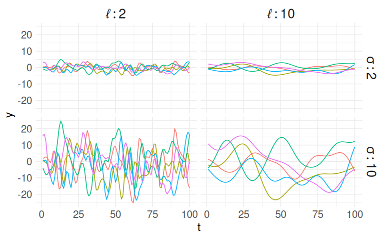
Squared Exponential
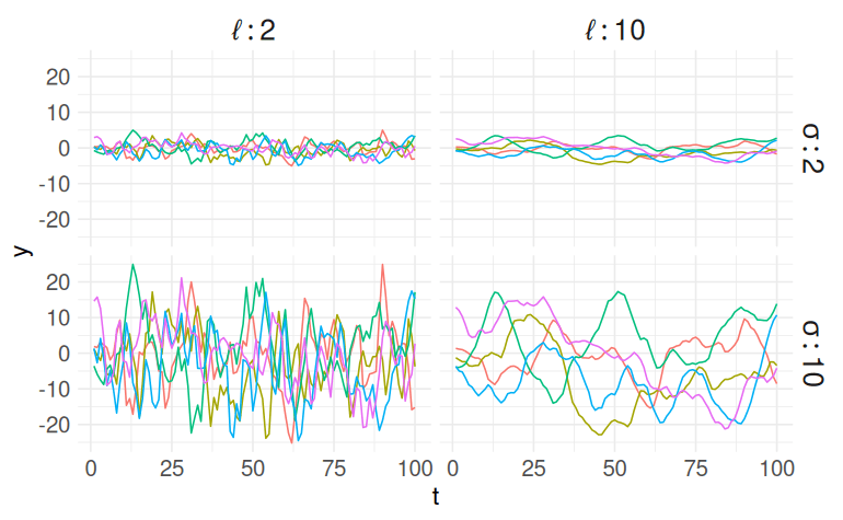
Matern 3/2
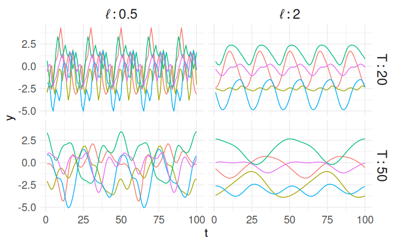
Periodic
\tau = | t_r - t_c |; \sigma, \ell, T > 0
$$\kappa(\tau; \sigma, \ell) = \sigma^2 \exp\left\{ -\frac{1}{2}\left( \frac{\tau}{\ell}\right)^2\right\}$$
$$\kappa(\tau; \sigma, \ell) = \sigma^2 \left( 1 + \sqrt{3}\frac{\tau}{\ell}\right) \exp\left\{ - \sqrt{3} \frac{\tau}{\ell}\right\}$$
$$\kappa(\tau; \sigma, \ell, T) = \sigma^2 \exp\left\{ -\frac{2}{\ell^2} \sin^2\left( \pi \frac{\tau}{T}\right)\right\}$$
Squared Exponential Kernel
\kappa(\tau; \sigma, \ell) = \sigma^2 \exp\left\{ -\frac{1}{2}\left( \frac{\tau}{\ell}\right)^2\right\}
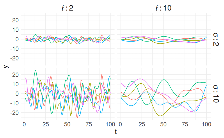
\tau = | t_r - t_c | \\
\sigma, \ell > 0
Bayesian Hierarchical Model
\begin{gather*}
i, r,c = 1, \dots, n.\\
\boldsymbol\theta = (\sigma_\mathrm{SE}, \ell_\mathrm{SE}, \sigma_\mathrm{M32}, \ell_\mathrm{M32}, \sigma_\mathrm{P}, \ell_\mathrm{P}, T)
\end{gather*}
\begin{align*}
[\boldsymbol\Sigma]_{r,c} &= \kappa(t_r - t_c \mid \boldsymbol{\theta})\\
&= \kappa_1(\tau; \sigma_\mathrm{SE}, \ell_\mathrm{SE}) + \kappa_2(\tau; \sigma_\mathrm{M32}, \ell_\mathrm{M32}) + \kappa_3(\tau; \sigma_\mathrm{P}, \ell_\mathrm{P}, T)
\end{align*}
Squared Exponential
Matern 3/2
Periodic
\(S_i \sim \mathcal{N}\left(f_i, \hat{e_i}^2\right)\)
\(\boldsymbol{f} \sim \mathcal{GP}\left(\boldsymbol{0}, \boldsymbol{\Sigma}_{n \times n}\right)\)
Hyperparameters
Flux density
GP prior
Bayesian Hierarchical Model
S_i \sim \mathcal{N}(f_i, \hat{e}_i^2), \qquad i = 1, \dots, n.
\boldsymbol{f} \sim \mathcal{GP}(\boldsymbol{0}, \boldsymbol{K}_{n \times n})
\begin{split}
[K]_{r,c} = \kappa(t_r,t_c \mid \boldsymbol{\theta}) =~& \sigma^2_\textrm{SE}\, \exp\left\{-\frac{1}{2}\frac{(t_r - t_c)^2}{\ell_\textrm{SE}^2}\right\} + \\
& \sigma^2_\textrm{M32} \left( 1 + \sqrt{3}\,\frac{|t_r - t_c|}{\ell_\textrm{M32}}\right) \exp\left\{-\sqrt{3}\frac{|t_r - t_c|}{\ell_\textrm{M32}}\right\} + \\
& \sigma^2_\textrm{P}\, \exp\left\{-\frac{2}{\ell_\textrm{P}^2} \sin^2\left( \pi\frac{|t_r - t_c|}{T}\right)\right\}, \qquad r,c = 1, \dots, n.
\end{split}
\begin{gather*}
\sigma_\textrm{SE}, \sigma_\textrm{M32},\sigma_\textrm{P} \sim \mathcal{N}^+(0,1) \\
\ell_\textrm{SE}, \ell_\textrm{M32}, \ell_\textrm{P} \sim \mathrm{InvGamma}\left(\alpha = 3, \beta = \frac{1}{2} \times \lceil\textrm{range}(t)\rceil\right) \\
T \sim \mathrm{Uniform}\left(2 \times \textrm{min}(\Delta t), \frac{1}{2} \times \textrm{range}(t)\right) \\
\ell_\textrm{SE}, \ell_\textrm{M32},\ell_\textrm{P} > \textrm{min}(\Delta t) \\
\ell_\textrm{SE} > \ell_\textrm{M32} \\
\end{gather*}
Data model
Process model
Parameter model
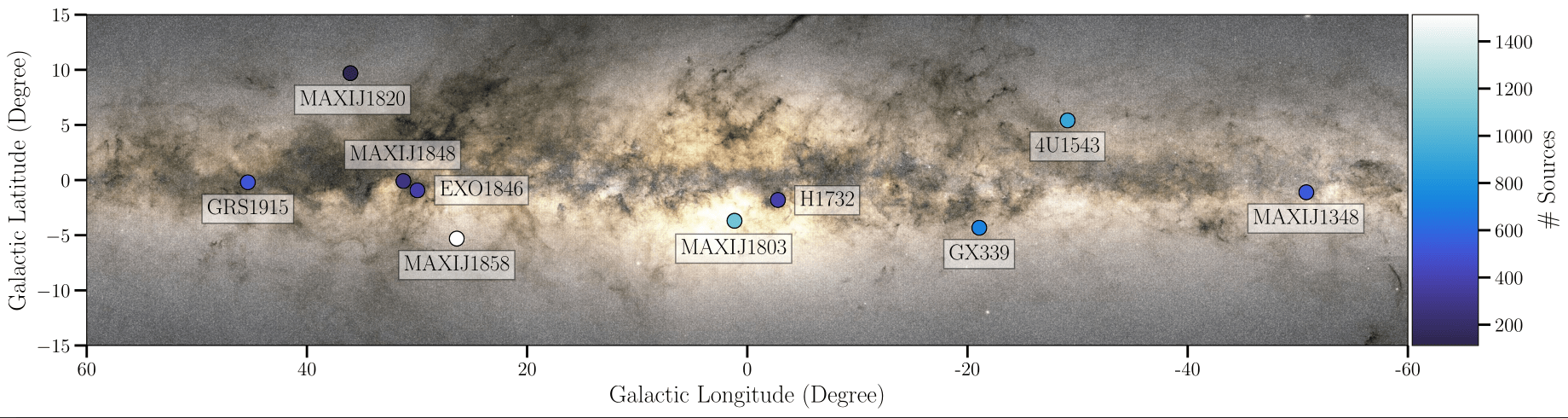
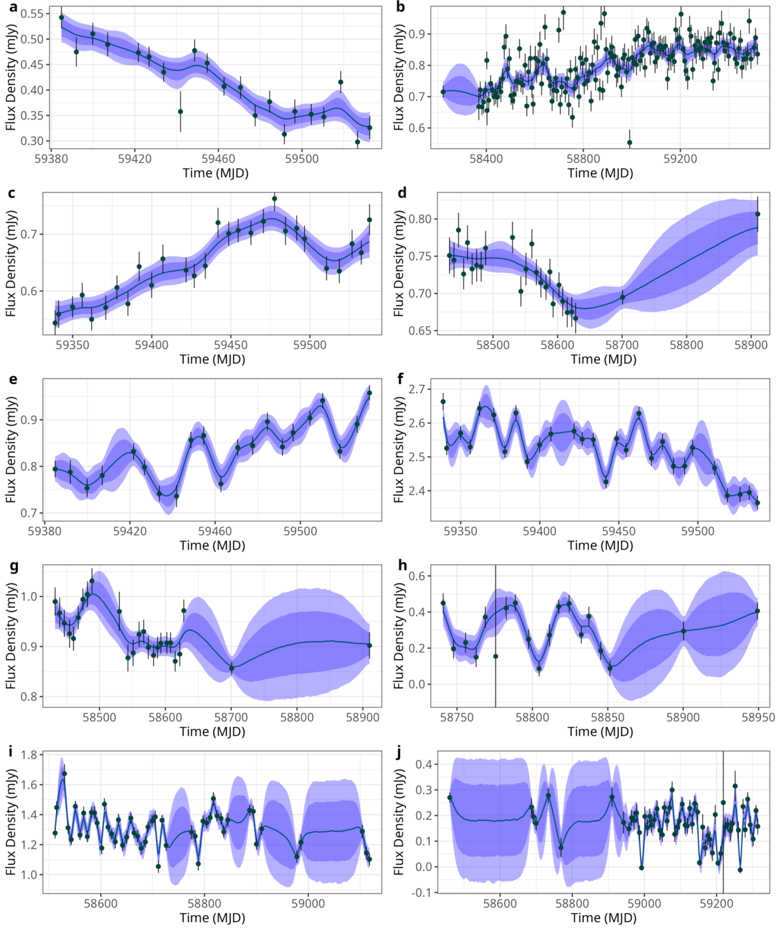
ThunderKAT Survey
- MeerKAT image domain transients survey
- Field-of-view of \(\approx 1^\circ \)
- 5,371 radio live curves over 10 fields
- Flux density and standard errors
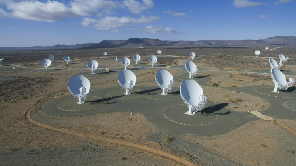
MeerKAT (Source: SARAO)
7D Hyperparameterspace
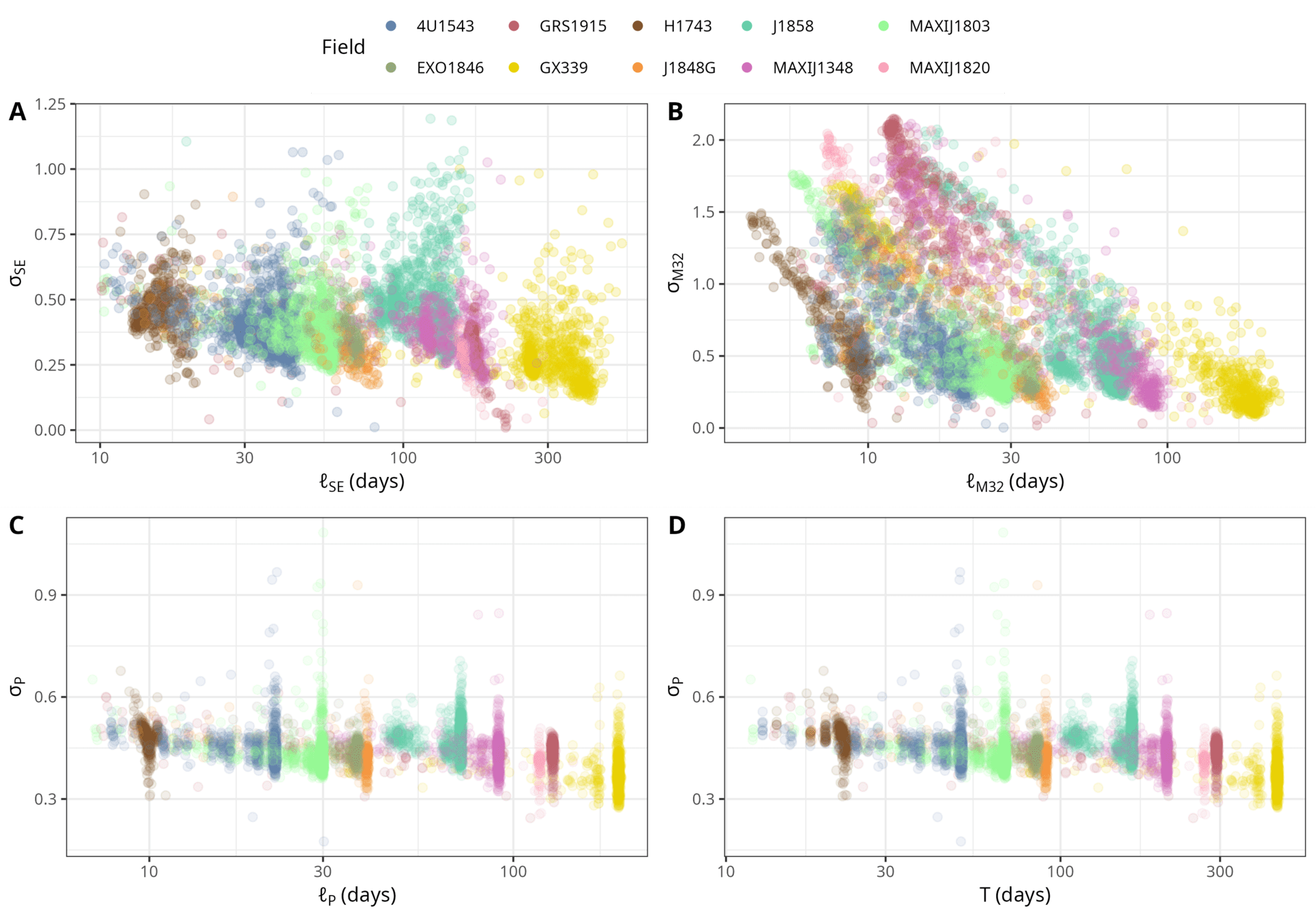
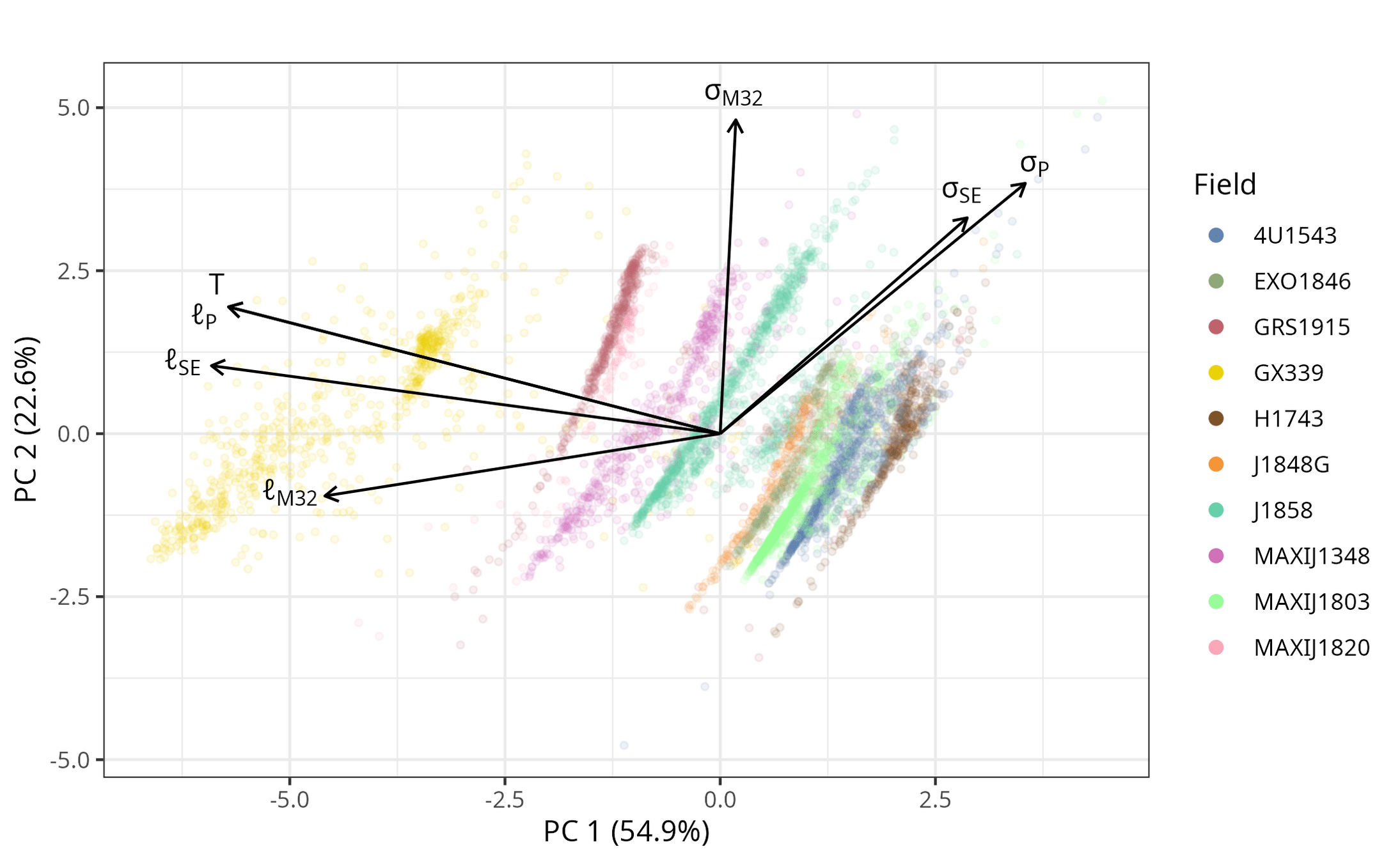
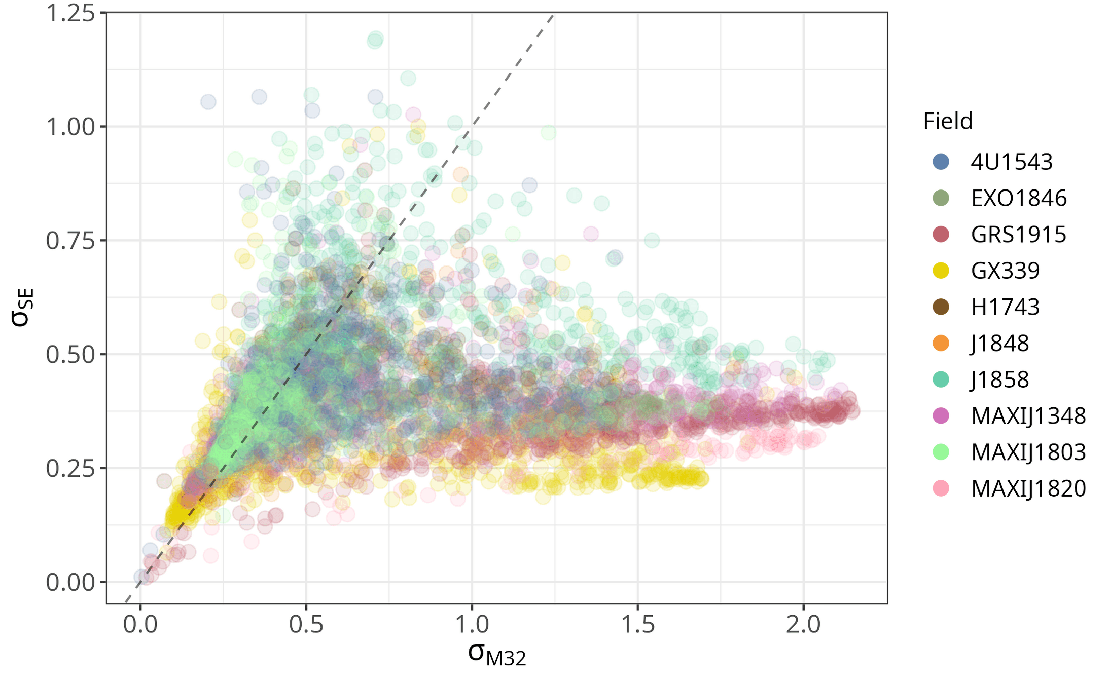
Amplitude Hyperparameters
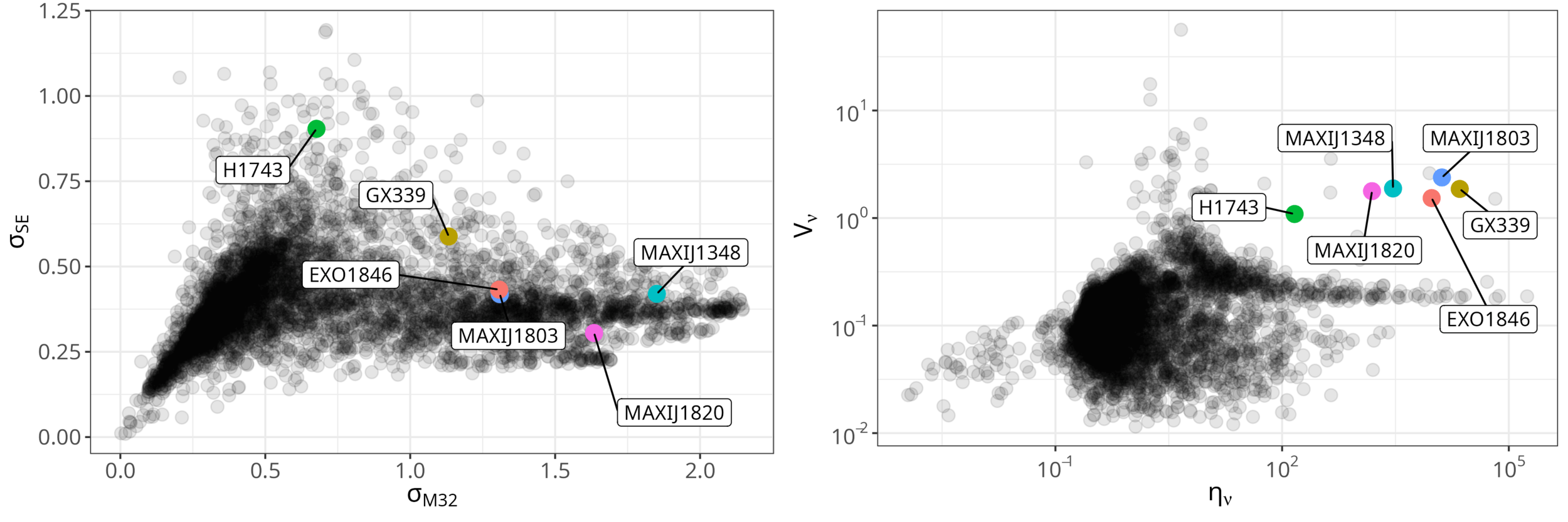
Interpeting Amplitude as Transience
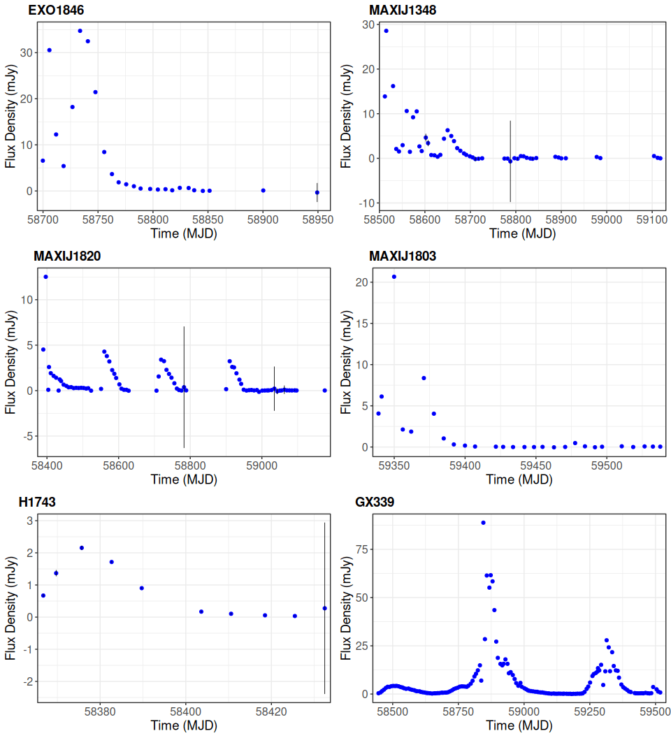
- Transience seems to manifest as large values in amplitude, \(\sigma_\mathrm{SE}\), \(\sigma_\mathrm{M32}\).
- Previously identified transient and variable candidates by Andersson et al. (2023) all seem to lie in the upper right of this 2D hyperparameter subspace.
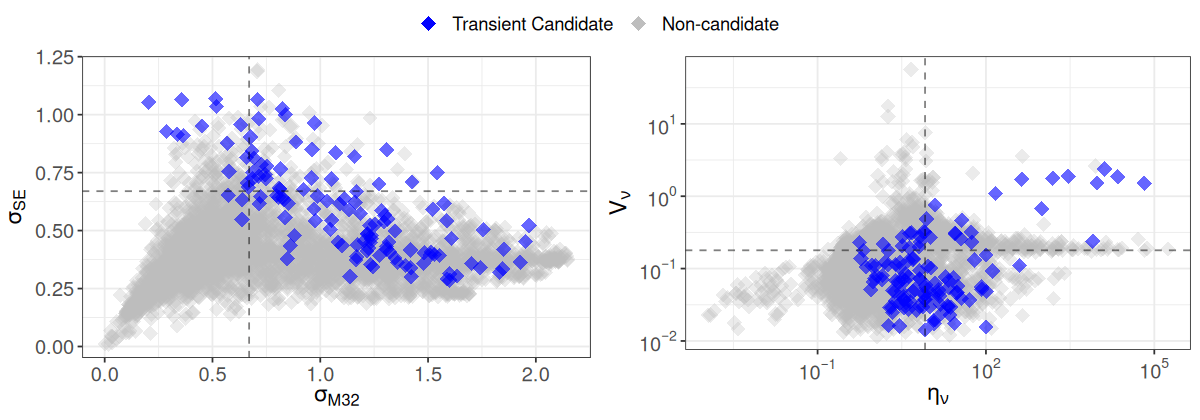
Data: Andersson et al. (2023)
Figure: Fu et al. (under review)
\( (\eta_\nu, V_\nu) \) vs. \( (\sigma_\mathrm{M32}, \sigma_\mathrm{SE})\)
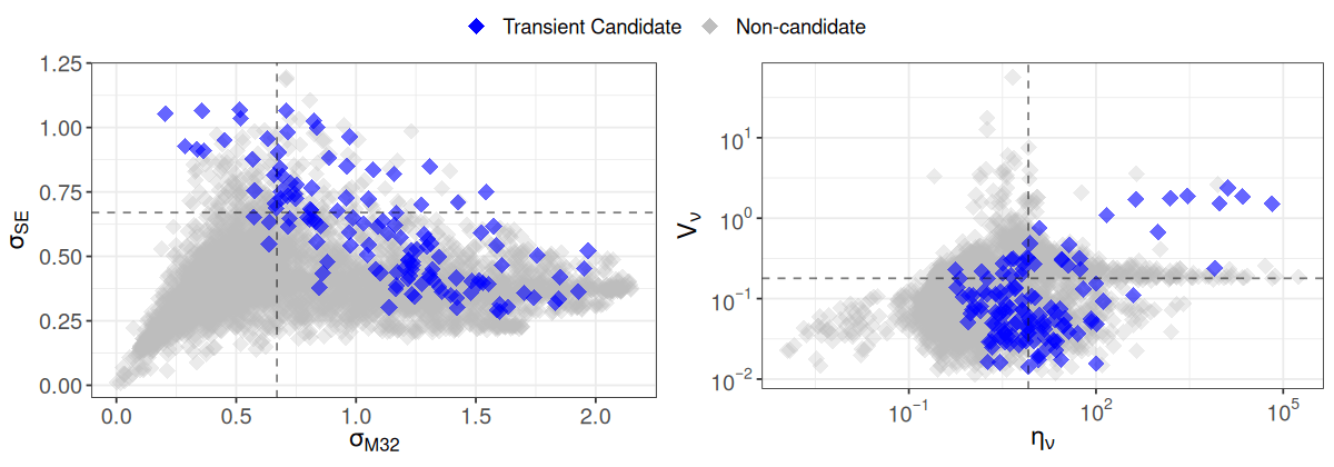
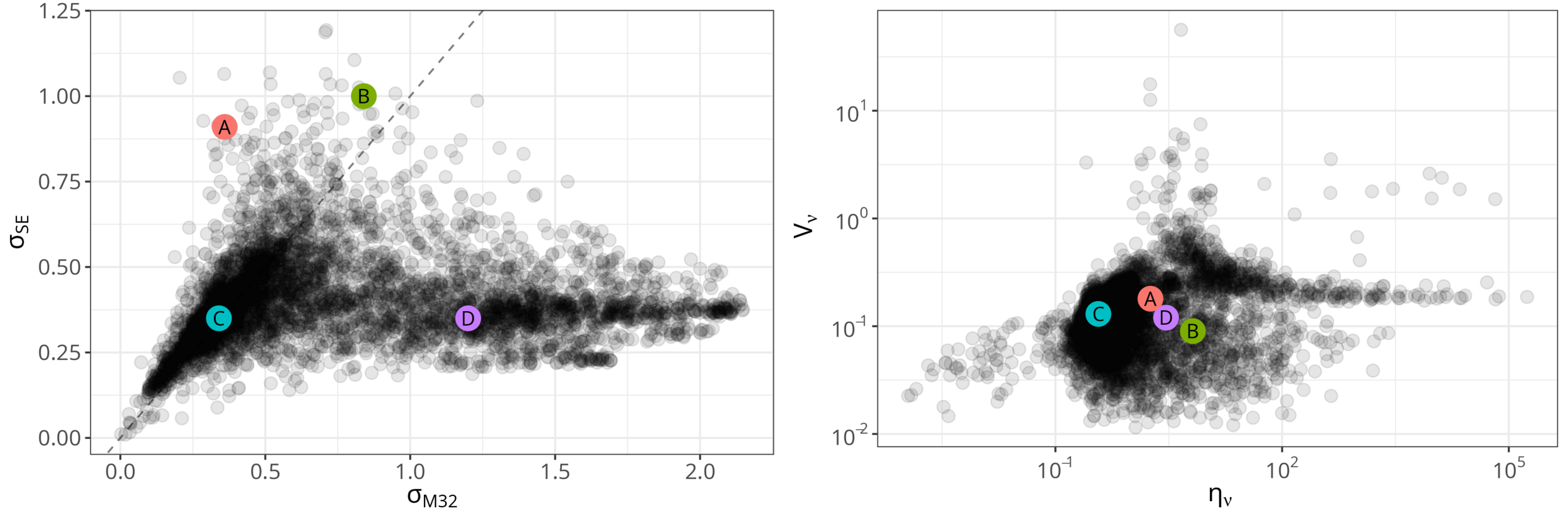
Parameterspace
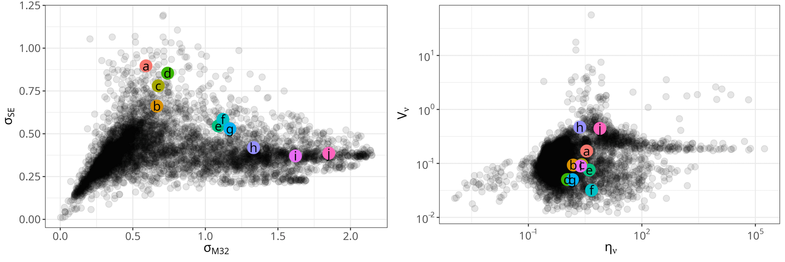
\( (\eta_\nu, V_\nu) \) vs. \( (\sigma_\mathrm{M32}, \sigma_\mathrm{SE})\)
NN Candidates
Robust characterisation of transient radio light curves using Gaussian process regression
By Shih Ching Fu
Robust characterisation of transient radio light curves using Gaussian process regression
The advent of large-scale surveys that observe thousands, if not millions, of sources puts the task of identifying novel candidates beyond the manual capability of astronomers. To automate the sifting of these sources at scale, a statistical approach can be used to characterise and classify promising candidates. Care must be taken, however, to not overfit to a particular object type or survey configuration so that processing can be applied across surveys without introducing statistical biases. In this work, I present a Gaussian process (GP) regression approach for statistically characterising light curves and demonstrate this approach on 5131 radio light curves from the ThunderKAT survey. The benefits of a GP approach include the implicit handling of data sparsity and irregular sampling, accommodating light curves of diverse shapes, and having astrophysically meaningful interpretations of the fitted model hyperparameters. Indeed, I found distinct regions in the amplitude hyperparameter space that point to a candidate's propensity to be a transient or variable source. Compared with variability metrics commonly used in radio astronomy, this approach has improved discriminatory power.